• Chapter 2. Statistical Learning
• 2.1. What is Statistical Learning?
  • 2.1.1. Why Estimate $f$ ?
    • Prediction
    • Inference
  • 2.1.2. Estimating $f$ : By Using Training Data
    • Parametric Methods: Model-based approach
    • Non-parametric Methods: Data-driven approach
    • Example of Nonparametric model: KNN Reg.
  • 2.1.3. Trade-off between Prediction Accuray & Interpretability
  • 2.1.4. Supervised Vs. Unsupervised Learning
  • 2.1.5. Regression Vs. Classification Problems
• 2.2. Assessing Model Accuracy
  • 2.2.1. Measuring the Quality of Fit
    • Mean squared error (MSE)
  • 2.2.2. Bias-Variance Trade-off
    • Trade-off in KNN Reg.
  • 2.2.3. The Classification Setting
    • The Bayes Classifier - Two-class Problem
    • K-Nearest Neighbors (KNN)

Chapter 2. Statistical Learning

2.1. What is Statistical Learning?

• Format of Statistical Learning:
  $ Y=f(X)+\epsilon $
  assume a relationship between $Y$ and $X$;
  $Y$: observed quantitative response
  $X$: $p$ different predictors $(X_1, X_2, \ldots , X_p)$
  $f$ : Fixed but UNKNOWN function of predictors $X$
  $\epsilon$ : a random error term, independent of $X$ which has mean zero; $E(\epsilon)=0$
  $\rightarrow$ Statistical Learning: A set of methods estimating $f$.

2.1.1. Why Estimate $f$ ?

• Why do we estimate $f$ ?
  1) Prediction: $Y$
  2) Inference: Relationship between $X$ & $Y$

Prediction

• $\text{Prediction of } \; Y : \hat{Y} = \hat{f}(X)\quad (\hat{f} : \text{Estimate of }f) $
  $\text{Accuracy of } \; \hat{Y} \text{ depends on reducible & irreducible errors}$;

• with a given(fixed) estimate $\hat{f}$ and a set of predictors $X$,
  while true function $f$ is also fixed from definition,
  \(\underbrace{E[Y-\hat{Y}]^2}_{MSE} = \underbrace{[f(X)-\hat{f}(X)]^2}_{\text{reducible error}} + \underbrace{Var(\epsilon)}_{\text{irreducible error}}\)

• derivation
  \(\begin{align*} E[Y-\hat{Y}]^2 &= E\left[\{f(X)+\epsilon\} - \hat{f}(X) \right]^2 \\ &= E\left[ \{f(X)-\hat{f}(X)\}^2 + 2 \epsilon \ (f(X)-\hat{f}(X)) + \epsilon^2 \right] \\ &= E\left[\{f(X)-\hat{f}(X)\}^2\right] + 2E[\epsilon]\cdot E\left[f(X)-\hat{f}(X)\right] + E[\epsilon^2] \\ & \quad \quad \scriptstyle f, \hat{f} \text{ and } X \text{ are fixed, } E(\epsilon)=0 \text{ and } E(\epsilon^2)\ =\ Var(\epsilon) \\ &= [f(X)-\hat{f}(X)]^2 + Var(\epsilon) \end{align*}\)

• Reducible error : controlable, can be reduced by selecting a better model Irreducible error: uncontrolable, nature of data

Inference

• interested in: Which predictors are associated with the response?
  What is the relationship between the response and each predictor?
  Can the relationship between Y and each predictor be adequately summarized
  using a linear equation, or is the relationship more complicated?

• Characteristics of linear & nonlinear models:
  1) Linear : Relatively Simple & interpretable inference but poor prediction
  (when true function $f$ is nonlinear)
  2) Nonlinear : More accurate but difficult to interpret
  $\rightarrow$ Depends on your Goal of analysis

2.1.2. Estimating $f$ : By Using Training Data

• Estimation Methods:
  1) Parametric: Assume specific function $f$ (linear&non- both)
  2) Non-parametric: No Assumption; Data-driven method (nonlinear)

Parametric Methods: Model-based approach

• Step 1: Assumption about the functional form of $f$
  Training data consist of n obs. {$(x_1,y_1), (x_2,y_2), \ldots , (x_n,y_n)$}
  where $x_i = ( x_{i1}, x_{i2}, \ldots , x_{ip} ) ^T$
  with $ \scriptstyle\text{(p+1)} $ coefficients $\ \beta_0, \beta_1, \ldots, \beta_p$
  $\rightarrow $ linear form $ f(X)= \beta_0 + \beta_1X_1 + … + \beta_pX_p$

• Step 2: Estimate Parameters
  $Y \approx \hat{\beta}_0 + \hat{\beta}_1X_1 + … + \hat{\beta}_pX_p = \hat{f}(X)$
  $\rightarrow $ approaches to fitting model

• Advantage:
  Simplifies the problem of estimating $f$ to estimating a set of parameters

• Disadvantage: Specific form of $f$
  Not match with the true $f$: poor estimation & poor prediction
  $\rightarrow\;$ Flexible parametric model : model with more parameters
  • Flexible model $\equiv$ Complex model
    but overfitting problem still remains:
    models could follow errors or noises, too closely
• Underfitting vs Overfitting problems
  underfit: estimation has not enough accuracy, miss to capture the true structure
  overfit: more complexity than true $f$

Non-parametric Methods: Data-driven approach

• No assumptions about functional form of $f$
  $\Rightarrow $ potential to accurately fit a wider range of possible shapes of $f$
• Disadvantage:
  1) Large number of obs. are required to get an accurate $f$ relative to a parametric method
  2) Overfitting $\Leftrightarrow$ Level of smoothness; Model complexity
  (how to determine it?)

Example of Nonparametric model: KNN Reg.

• Idea: Similar inputs have Similar outputs
  Step: when predicting $\hat{Y}_0$ with input $X_0$
  • 1) Determine $K$ (level of smoothness)

  • if K==N: Y = Var(Y)
    if K==1: Y = perfect fit; no training error

  • 2) find $K$ closest training obs. from the target input point($X_0$) using Euclidean distance

  • 3) average of these #k Y values
    \(\rightarrow\hat{Y}_0 = \frac{1}{K}\sum_{x_i\in \mathcal N}^K y_i\)
• Effect of $K$ (tuning parameter/ model flexibility parameter)
  • decides the level of smoothness (under or overfitting)
  • As $K \uparrow \; \Rightarrow \text{flexibility} \downarrow$ : the fitted line is simple
  • As $K \downarrow \; \Rightarrow \text{flexibility} \uparrow$ : the fitted line is wiggly

2.1.3. Trade-off between Prediction Accuray & Interpretability

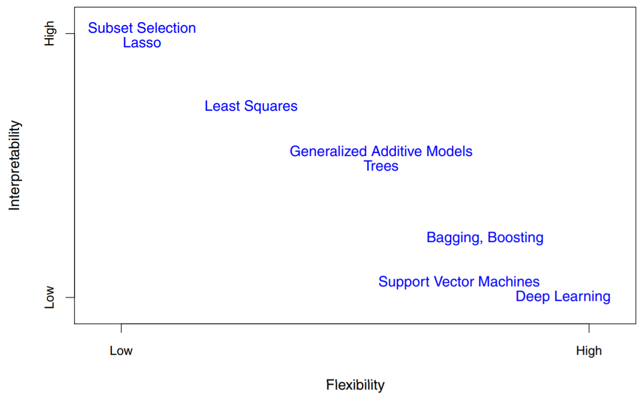
• tradeoff between flexibility and interpretability

• based on our goal:
  inference ($\rightarrow$ restrictive model)
  prediction ($\rightarrow$ flexible model)
  BUT NOT ALWAYS THE CASE

2.1.4. Supervised Vs. Unsupervised Learning

• Supervised:
  for each observation $x_i$, there is an associated response measurement $y_i$
  goal is to fit a model, to predict or interpret(inference)

• Unsupervised:
  no associated response $y_i$, not possible to fit a model, no response to predict
  goal is to understand the relationships between the variables or between the observations

2.1.5. Regression Vs. Classification Problems

• Variables either quantitative or qualitative(categorical)
• Different models can be used on both problem

2.2. Assessing Model Accuracy

• Evaluate the performance of models on a given dataset and Select the best model
• Criterions, e.g. Better prediction of $Y$

2.2.1. Measuring the Quality of Fit

Mean squared error (MSE)

• Training MSE = \(\frac{1}{n} \sum_{i=1}^n (y_i - \hat{f}(x_i))^2\)
  the most commonly-used measure in the regression setting
  can be used for building model, but is not our interest;
  cannot be a measure for model selection

• when training RSS = \(\sum(y_i - \hat{y_i})^2\), MSE = \(\frac{RSS}{N}\)
  \(R^2 = 1 - \frac{RSS}{TSS}\)
  • as more $X$ variables added, even $X$ are not important predictors,
  • RSS & MSE decrease and $R^2$ increases, regardless of existence of test data
• Test MSE \(= \frac{1}{m}\sum_{i=1}^m(y_i^0 - \hat{f}(x_i^0))^2\)
  with unseen test observation not used to train,
  Select model that gives the lowest test MSE.
  • Test MSE(error rate) is always larger than Training MSE;
    We estimated model function $f$ to minimize its training error
  • if there’s NO test data: Sample re-use methods
    (e.g., bootstrap, cross-validation)
• for Classification problem: Misclassification rate

2.2.2. Bias-Variance Trade-off

• expected test MSE($\scriptstyle\text{ideal measure}$)= $E[y_0-\hat{f}(x_0)]^2$ when $(x_0,y_0)$ is a test obs.

• in population: #K training sets and #K function $f_k$
  Estimation of expected test MSE: \(\\ \hat{E}[y_0 - \hat{f}(x_0)]^2 = \frac{1}{K} \sum_{k=1}^K[y_0-\hat{f}_k(x_0)]^2\)

• derivation
  For given $x_0$, (when $\epsilon$ is irreducible error) \(\\ \begin{align*} \hat{E}[y_0 - \hat{f}(x_0)]^2 &= E [ \{ y_0 -E(\hat{f}(x_0)) \} - \{ \hat{f}(x_0) - E(\hat{f}(x_0)) \} ]^2 \\ (1) \cdots &= E [ y_0 -E(\hat{f}(x_0)) ] ^2 \\ (2) \cdots & \; + E [\hat{f}(x_0) - E(\hat{f}(x_0)) ] ^2 \\ (3) \cdots & \; - 2E[ \{ y_0 -E(\hat{f}(x_0)) \} \{ \hat{f}(x_0) - E(\hat{f}(x_0)) \} ] \end{align*}\)

• (1) \(\\ \begin{align*} &= E [(f(x_0) + \epsilon - E(\hat{f}(x_0)) ] ^2 \\ &= E[ f(x_0)^2 +\epsilon^2 + [E(\hat{f}(x_0)) ]^2 + 2f(x_0)\epsilon -2f(x_0)E(\hat{f}(x_0)) - 2\epsilon E(\hat{f}(x_0)) ] \\ & \quad \scriptstyle\text{when } E(\epsilon) \text{ goes to } 0 \\ &= E[E(\hat{f}(x_0)) - f(x_0)] ^2 + E(\epsilon^2) \\ & \quad \scriptstyle{f(x_0) - E(\hat{f}(x_0)) - \text{ is a Bias}} \\ &= [Bias(\hat{f}(x_0))]^2 + Var(\epsilon^2) \end{align*}\)

• (2) = $Var(\hat{f}(x_0)); $ model variance($\scriptstyle\text{different fit’s from randomness of training sets}$)
• (3) = 0

$\therefore \hat{E}[y_0 - \hat{f}(x_0)]^2 = Var(\hat{f}(x_0)) + [Bias(\hat{f}(x_0))]^2 + Var(\epsilon) $

• $Var(\hat{f}(x_0)$ : model variance

• $ [Bias(\hat{f}(x_0)]$: Systematic model error
  (caused by model assumptions; e.g. true f: nonlinear)

• $ Var(\epsilon)$ : Irreducible error

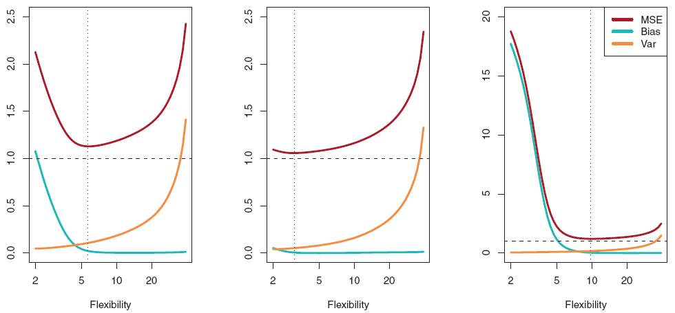
Model Flextibility $\uparrow$ $\Rightarrow$ model variance $\uparrow$ & model bias $\downarrow$
Model Flextibility $\downarrow$ $\Rightarrow$ model variance $\downarrow$ & model bias $\uparrow$

$\rightarrow$ optimal model flextibility is different for each datasets

Trade-off in KNN Reg.

• given $Y = f(X) + \epsilon$, $E(\epsilon) = 0 $ and $Var(\epsilon) = \sigma^2$

• Expected test MSE at $x_0$:
  \(E[ (Y- \hat{f_k}(x_0) )^2 | X = x_0 ] = Var(\hat{f}(x_0)) + [Bias(\hat{f}(x_0))]^2 + Var(\epsilon)\)

• (1) \(\\ \begin{align*} Var(\hat{f_k}(x_0)) &= Var(\frac 1 K \sum_{i \in \mathcal N (x_0)} Yi )\\ &= \frac 1 {K^2} \sum Var( Yi ) \\ &= \frac 1 {K^2} \sum Var( f( x_i) + \epsilon_i ) \\ &= \frac 1 {K^2} \sum \sigma^2 = \frac 1 {K^2} \cdot K \cdot \sigma^2 = \frac {\sigma^2} K \end{align*}\)

• (2) \(\\ \begin{align*} Bias(\hat{f_k}(x_0)) &= f(x_0) - E(\hat{f}(x_0)) \\ &= { f(x_0) - E[\frac1 K \sum_{i \in \mathcal N (x_0)} ^ K Y_i ] } \\ &= { f(x_0)- \frac 1 K \sum E (f(x_i)+\epsilon_i)} \\ &= f(x_0) - \frac 1 K \sum E (f(x_i) \\ \end{align*}\)

\(\therefore\) Expected test MSE = \(\sigma ^2 + [f(x_0) - \frac{1}{K}\sum_{x_i \in \mathcal N (x_0)}^k f(x_i) ]^2 + \frac {\sigma^2}{K}\)

• when we use large number of K - as K increases,
  model complexity and model variance decreases, then bias increases;
  which is a simpler model.

2.2.3. The Classification Setting

• training misclassification rate \(= \frac 1 n \sum_{i=1}^n I(y_i \not = \hat y_i )\)
  $\hat y_i$: $i_{th}$ observation using $\hat f$
  $I(y_i \not = \hat y_i )$: indicator variable that;
  1 if $y_i \not = \hat y_i$ and 0 if $y_i = \hat y_i$

• test error = $ Ave(I(y_0 \not = \hat y_0))$ where;
  $\hat y_0$ is the predicted class label for the test observation with predictor $x_0$

The Bayes Classifier - Two-class Problem

• Assign a test observation with predictor vector $x_0$ to the class $j$ for which;
  conditional probability $Pr(Y=j|X=x_0)$ is largest.
  with only two possible response values, say class 1 or class 2,
  predict class 1 if $Pr(Y=1|X=x_0)$ > 0.5, and class 2 otherwise.

• Bayes error rate
  for choosing the largest $Pr(Y=j|X=x_0)$,
  the error rate will be $\ 1 - max_j Pr(Y=j|X=x_0)$ at $X=x_0$

  • Overall Bayes error rate = \(1 - E\left[max_j Pr(Y=j|X) \right]\)
    expectation averages the probability over all possible values of X

K-Nearest Neighbors (KNN)

• \(Pr(Y=j|X=x_0) = \frac{1}{K}\sum_{i \in \mathcal{N}_0} I(y_i=j)\)
  conditional probability for class j
  $\mathcal{N}_0$: K points in the training data that are closest to $x_0$
  KNN classifies the test obs. to the class with the largest probability.