So far: recurrent models for (most) NLP

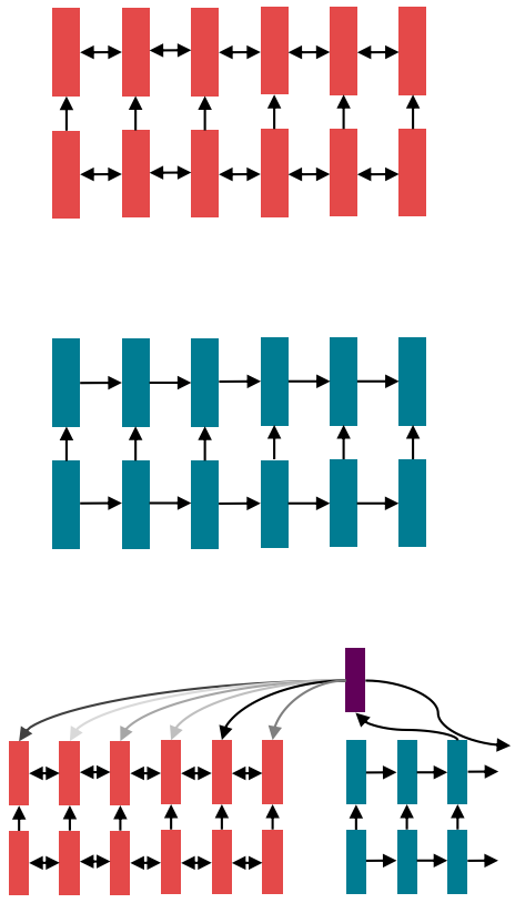
- Circa 2016, the de facto strategy in NLP is to encode sentences with a bidirectional LSTM.
(for example, the source sentence in a translation)



- Define your output (parse, sentence, summary) as a sequence, and use an (unidirectional) LSTM to generate it.




- Use attention to allow flexible access to memory.

• Seq2Seq models need to process variable-length inputs into fixed-length representations

• To deal with seq2seq problems, we learned end-to-end differentiable system using an encoder-decoder architecture.

• Instead of entirely new ways of looking at problems, we’re trying to find the best building blocks to plug into our models and enable broad progress.

Issues with recurrent models: Linear interaction distance

• RNNs are unrolled “left-to-right”:
  This encodes linear locality: a useful heuristic
  • Nearby words often affect each other’s meanings
• Problem: RNNs take O(sequence length) steps for distant word pairs to interact.
  
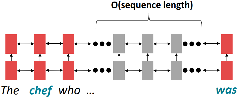
  • Hard to learn long-distance dependencies (because gradient problems)
  • Linear order of words is “baked in”; linear order isn’t the right way to think about sentences

Issues with recurrent models: Lack of parallelizability

• Forward and backward passes have O(sequence length) unparallelizable operations
  • Future RNN hidden states can’t be computed in full before past RNN hidden states have been computed; not GPU friendly, inhibits training on very large datasets.

Alternatives: Word windows

• Word window models aggregate local contexts (Also known as 1D convolution)
  • Number of unparallelizable operations does not increase sequence length
    (O(1) dependence in time)
    
• What about in long-distance dependencies?
  • Stacking word window layers allows interaction between farther words
  • Maximum Interaction distance = sequence length / window size
    But if your sequences are too long, you’ll just ignore long-distance context

Alternatives: Attention

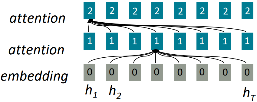
• Attention treats each word’s representation as a query to access and incorporate information from a set of values.
  • Out of the encoder-decoder structure; think about attention within a single sentence.
  • Number of unparallelizable operations does not increase sequence length; not parallelizable in depth but parallelizable in time.
  • Maximum interaction distance: O(1), since all words interact at every layer
    

Self-Attention

• Recall: Attention operates on queries, keys, and values.
  • queries: $q_1, q_2, \ldots, q_T \in \mathbb{R}^d$
  • keys: $k_1, k_2, \ldots, k_T \in \mathbb{R}d$
  • values: $v_1, v_2, \ldots, v_T \in \mathbb{R}d$

• In self-attention, the queries, keys, and values are drawn from the same source.
  For example, if the output of the previous layer is $x_1, \ldots, x_T$ (one vec per word), we could let $v_i = k_i = q_i = x_i$ (use the same vectors for all of them).

• The (dot product) self-attention operation is as follows:
  • Compute key-query affinities: $e_{ij} = q_i^T k_j $
  • Compute attention weights from affinities(softmax):
    \(\begin{align*} \alpha_{ij} = \frac{\exp(e_{ij})}{\sum_{j^\prime} \exp(e_{ij^\prime})} \end{align*}\)
  • Compute outputs as weighted sum of values
    \(\begin{align*} \text{output}_i = \sum_j \alpha_{ij}v_j \end{align*}\)
• Q: FCN vs Self-Attention?

Self-attention as an NLP building block

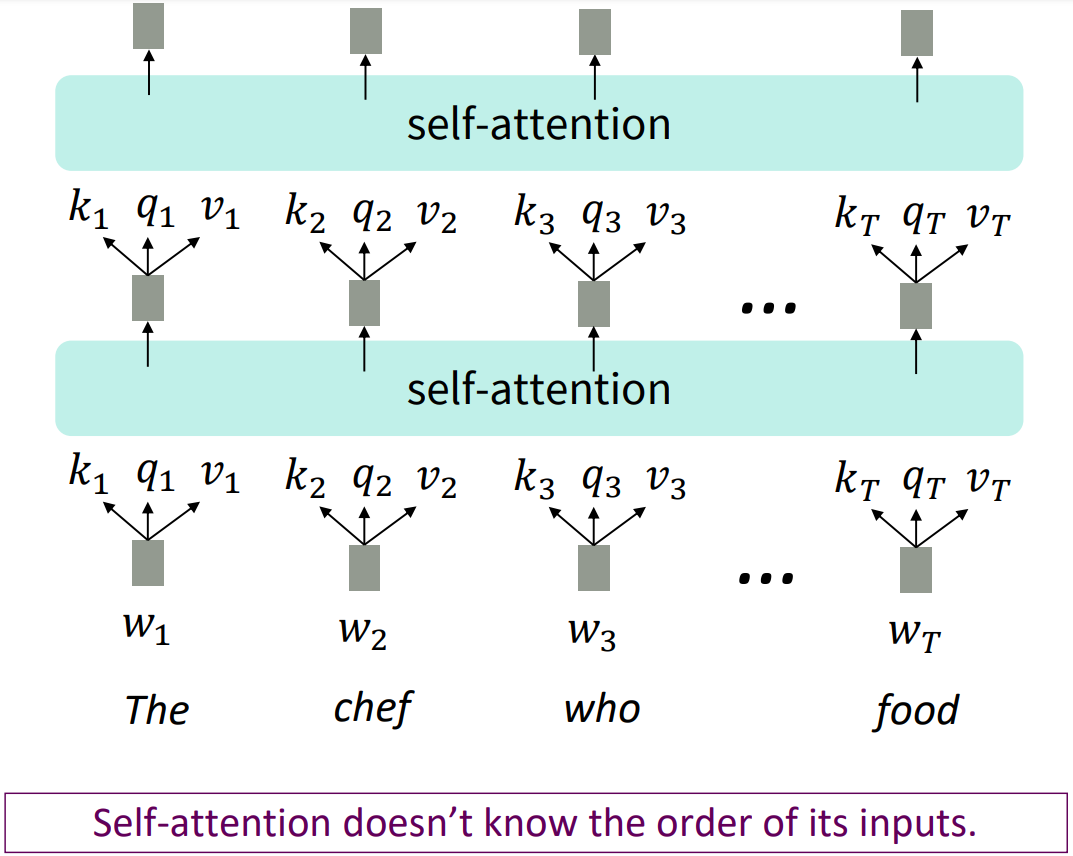
• Can self-attention replace the recurrence? NO.

Sequence order

• Self-attention is an operation on sets; it has no inherent notion of order.
  • To fix this, encode the order of the sentence.

• Consider representing each sequence index as a vector;
  $p_i \in \mathbb{R}^d$, for \(i \in \left\{ 1,2,\ldots, T \right\}\) are position vectors

• Let $\tilde{v}_i, \tilde{k}_i, \tilde{q}_i$ be our old inputs, then add $p_i$ to inputs;
  $v_i = \tilde{v}_i + p_i$
  $q_i = \tilde{q}_i + p_i$
  $k_i = \tilde{k}_i + p_i$
  • In deep self-attention networks, we do this at the first layer; you could concatenate them as well, but mostly, just add.

1. Position representation vectors through sinusoids
   • Sinusoidal position representations: concatenate sinusoidal functions of varying periods
     
   • Pros:
     • Periodicity indicates that maybe “absolute position” isn’t as important
     • Maybe can extrapolate to longer sequences as periods restart!
   • Cons:
     • Not learnable; also the extrapolation doesn’t really work!
2. Position representation vectors learned from scratch
   • Learned absolute position representations: Let a matrix $p \in \mathbb{R}^{d \times T}$ and each learnable parameters $p_i$ be a column of that matrix; Most systems use this!
   • Pros:
     • Flexibility: each position gets to be learned to fit the data
   • Cons:
     • Definitely can’t extrapolate to indices outside $1, \ldots, T$.
   • Some more flexible representations of position:
     • Relative linear position attention (Shaw et al., 2018)
     • Dependency syntax-based position (Wang et al., 2019)

Nonlinearities

• There are no elementwise nonlinearities in self-attention; stacking more self-attention layers just re-averages value vectors.

• Easy fix: add a feed-forward network to post-process each output vector.
  (Self-Att. - FF - Self-Att. - FF - ...)
  \(\begin{align*} m_i &= MLP(\text{output}_i) \\ &= W_2 \ast \text{ReLU}(W_1 \times \text{output}_i + b_1) + b_2 \end{align*}\)

Masking the future

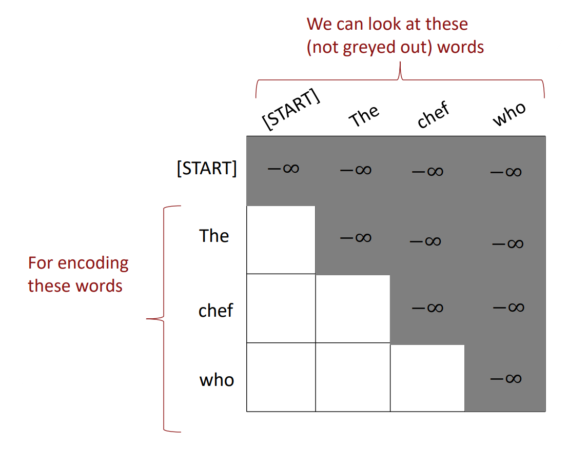
• To use self-attention in decoders, we need to ensure we don’t “look at the future” when predicting a sequence.

• Easily: at every timestep, we could change the set of keys and queries to include only past words. But it’s inefficient dealing with tensors, not parallelizable.

• Instead, to enable parallelization, mask out attention to future words by setting attention scores to $-\infty$ (attention weights to 0).
  $e_{ij} = \begin{cases} q_i^T k_j, & j < i
  -\infty, & j \ge i \end{cases}$
  

Recap: Necessities for a self-attention building block

• Self-attention: the basis of the method
• Position representations:
  Specify the sequence order, since self-attention is an unordered function of its inputs.
• Nonlinearities:
  At the output of the self-attention block, frequently implemented as a simple feed-forward network.
• Masking:
  In order to parallelize operations while not looking at the future, keeps information about the future from “leaking” to the past.

Transformer

• The Transformer Encoder-Decodr (Vaswani et al., 2017)
  At a high level look;

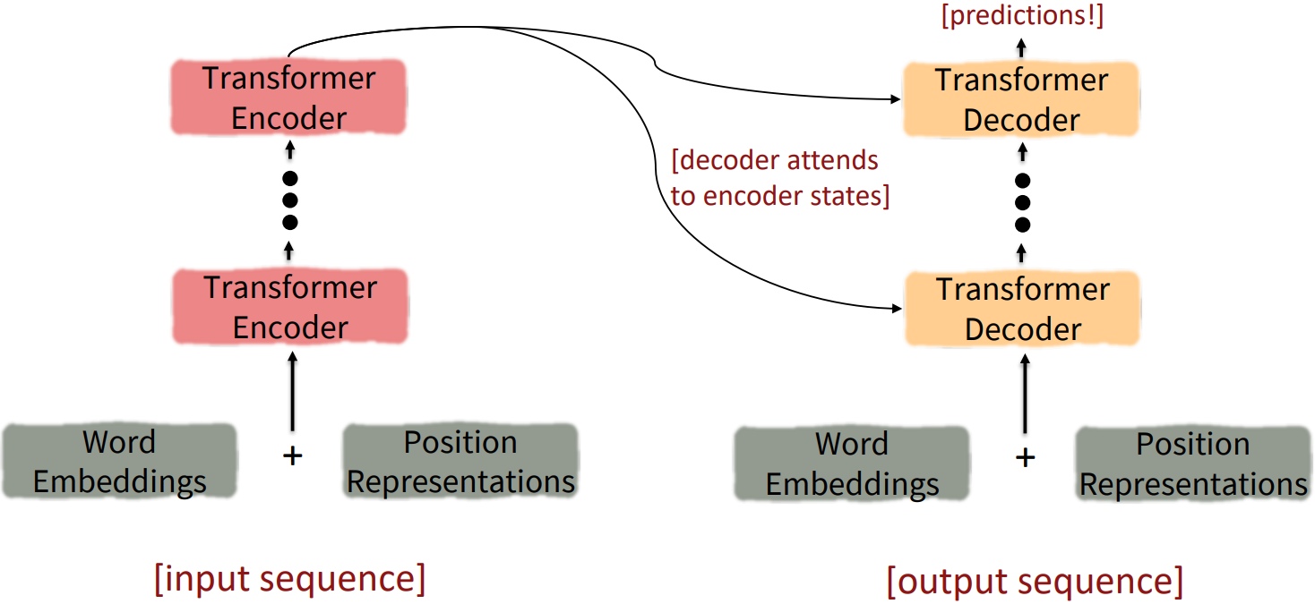
• What’s left in a Transformer Encoder Block:
  1. Key-query-value attention: How do we get input vectors from a single word embedding?
  2. __Multi-headed attention: Attend to multiple places in a single layer
  3. Tricks to help with training:
     • Residual connections
     • Layer normalization
     • Scaling the dot product These tricks don’t improve what the model is able to do; they help improve the training process. Both of these types of modeling improvements are very important.

The Transformer Encoder: Key-Query-Value Attention

• Let $x_1, \ldots, x_T \in \mathbb{R}^d$ be input vectors to the Transformer encoder. Then keys, queries, values are:
  • $k_i = Kx_i$, where $K \in \mathbb{R}^{d \times d}$ is the key matrix.
  • $q_i = Qx_i$, where $Q \in \mathbb{R}^{d \times d}$ is the query matrix.
  • $v_i = Vx_i$, where $V \in \mathbb{R}^{d \times d}$ is the value matrix.
    These matrices (of learnable parameters) allow different aspects of the $x$ vectors to be used/emphasized in each of the three roles.
• Computed in matrices,
  • Let $X = \left[ x_1; \ldots; x_T \right] \in \mathbb{R}^{T\times d}$ be the concatenation of input vectors.
  • First, note that $XK \in \mathbb{R}^{T\times d}$, $XQ \in \mathbb{R}^{T\times d}$, $XV \in \mathbb{R}^{T\times d}$.
  • The output tensor is defined as $\text{output} = \text{softmax}(XQ(XK)^T) \times XV$.

1. Take the query-key dot products in one matrix multiplication: $XQ(XK)^T = XQK^T X^T \in \mathbb{T}^{T\times T} $ (All pairs of attention scores)
2. Take softmax, and compute the weighted average with another matrix multiplication: $\text{output} \in \mathbb{T}^{T\times d}$

The Transformer Encoder: Multi-headed attention

• What if we want to look in multiple places in the sentence at once?
  • For word $i$, self-attention “looks” where $x_i^T Q^T K x_j$ is high, but maybe we want to focus on different $j$ for different reasons?
• Define multiple attention “heads” through multiple $Q, K, V$ matrices:
  • Let $Q_l, K_l, V_l \in \mathbb{R}^{d\times \frac{d}{h}}$, where $h$ is the number of attention heads, and $l$ ranges from $1$ to $h$.
  • Each attention head performs attention independently:
    $\text{output}_l = \text{softmax}(XQ_l K_l^T X^T) \ast X V_l \in \mathbb{R}^{d/h}$
  • Then combine the all outputs from the heads:
    $\text{output} = Y\left[ \text{output}_1; \ldots, \text{output}_h \right]$, where $Y \in \mathbb{R}^{d\times d}$.
  • Each head gets to “look” at different things and construct value vectors differently.
    

The Transformer Encoder: Residual connections [He et al., 2016]

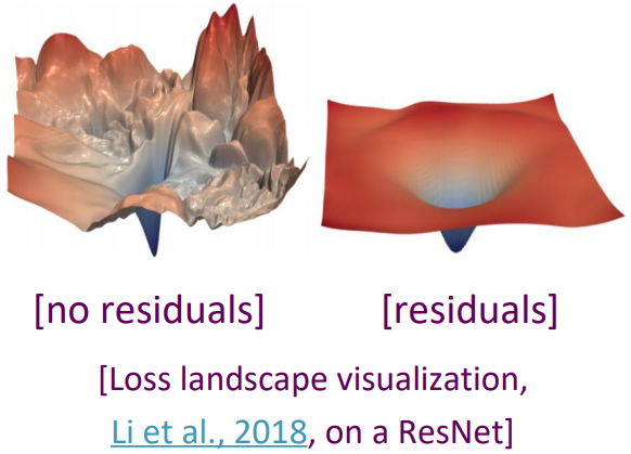
• Residual connections are a trick to help models train better.

• Instead of $X^{(i)} = \text{Layer}(X^{(i-1)})$ (where $i$ represents the layer)
  We let $X^{(i)} = X^{(i-1)} + \text{Layer}(X^{(i-1)})$ (so we only have to learn “the residual” from the previous layer)

• Solves vanishing gradient problem
• Residual connections are thought to make the loss landscape considerably smoother (thus easier training!)

The Transformer Encoder: Layer normalization [Ba et al., 2016]

• Layer normalization is a trick to help models train faster.
  • Idea: cut down on uninformative variation in hidden vector values by normalizing to unit mean and standard deviation within each layer.
  • LayerNorm’s success may be due to its normalizing gradients (Xu et al., 2019)
• Let $x\in \mathbb{R}^d$ be an individual (word) vector in the model.
  • Let the mean $\mu = \sum_{j=1}^d x_j \in \mathbb{R}$
  • Let the standard deviation $\sigma = \sqrt{\frac{1}{d}\sum_{j=1}^d (x_j-\mu)^2} \in \mathbb{R}$
  • Let $\gamma \in \mathbb{R}^d$ and $\beta \in \mathbb{R}$ be learned “gain” and “bias” parameters (Can omit)
  • Then layer normalization computes:
    \(\begin{align*}\text{output} = \frac{x-\mu}{\sigma + \epsilon}\ast\gamma + \beta \end{align*}\);
    (Normalize by scalar mean and variance, and modulate by learned elementwise gain and bias)

The Transformer Encoder: Scaled Dot Product [Vaswani et al., 2017]

• When dimensionality $d$ becomes large, dot products between vectors tend to become large.
  Because of this, inputs to the softmax function can be large, making the gradients small (leading to saturate region)

• Instead of the self-attention functiopn we’ve seen:
  $\text{output}_l = \text{softmax}(XQ_l K_l^T X^T) \ast X V_l$
  We divide the attention scores by $\sqrt{d/h}$, to stop the scores from becoming large just as a function of $d/h$ (The dimensionality divided by the number of heads.):
  $\text{output}_l = \text{softmax}(\frac{XQ_l K_l^T X^T}{\sqrt{d/h}}) \ast X V_l$

Now look at the Decoder Blocks

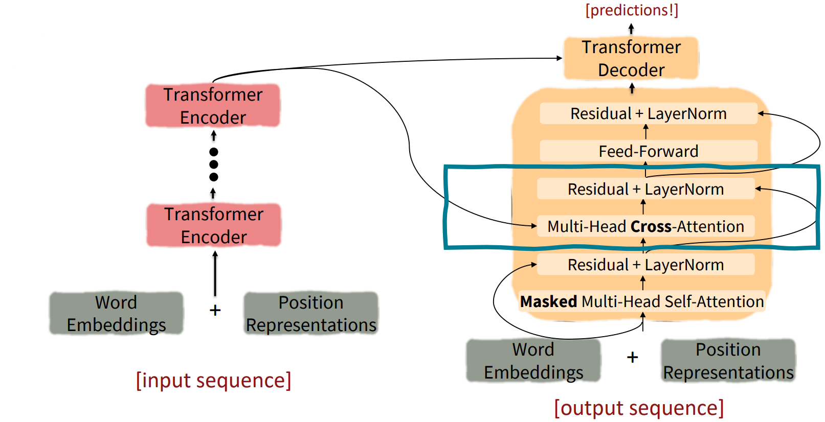
The Transformer Decoder: Cross-attention (details)

• Let $h_1, \ldots, h_T$ be output vecotrs from the Transformer encoder (the last block); $x_i \in \mathbb{R}^d$
  Let $z_1, \ldots, z_T$ be input vectors from the Transformer decoder, $z_i\in \mathbb{R}^d$
  Then keys and values are drawn from the encoder (like a memory); $k_i = Kh_i, v_i = Vh_i$
  The queries are drawn from the decoder; $q_i = Qz_i$

• In matrices:

  • Let $H = \left[ h_1; \ldots, h_T \right] \in \mathbb{R}^{T\times d}$ be the concatenation of encoder vecotrs.
  • Let $Z = \left[ z_1; \ldots, z_T \right] \in \mathbb{R}^{T\times d}$ be the concatenation of decoder vectors.
  • The output is defined as $\text{output} = \text{softmax}(ZQ(HK)^T)\times HV$.

What would we like to fix about the Transformer?

• Quadratic compute in self-attention:
  • Computing all pairs of interactions means our computation grows quadratically with the sequence length.
  • For recurrent models, it only grew linearly.
• Position representations:
  • Are simple absolute indices the best we can do to represent position?
  • Relative linear position attention (Shaw et al., 2018)
  • Dependency syntax-based position (Wang et al., 2019)

Quadratic computation as a function of sequence length

• One of the benefits of self-attention over recurrence was that it’s highly parallelizable.
  However, its total number of operations grows as $O(T^2 d)$, where $T$ is the sequence length, and $d$ is the dimensionality.

• Think of $d$ as around 1,000.
  So, for a single (shortish) sentence, $T \le 30; T^2 \le$ 900.
  In practice, we set a bound like $T = 512$.
  But what if we’d like $T\ge 10,000$? to work on long documents?

Recent work on improving on quadratic self-attention cost

• Considerable recent work has gone into the question,
  Can we build models like Transformers without paying the $O(T^2)$ all-pairs self-attention cost?

• Linformer (Wang et al., 2020)
  
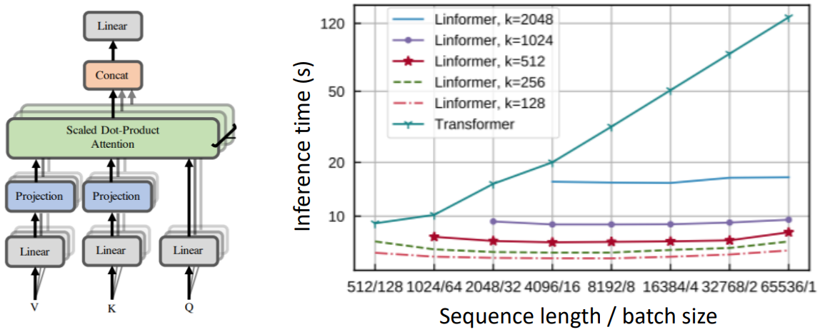
  • Key idea: map the sequence length dimension to a lower-dimensional space for values, keys.
• BigBird (Zaheer et al., 2021)
  
  • Key idea: replace all-pairs interactions with a family of other interactions, like local windows, looking at everything, and random interactions.