New Task: Machine Translation

Pre-Neural Machine Translation

Machine Translation (MT) is the task of translating a sentence x from one language (the source language) to a sentence y in another language (the target language).

1990s-2010s: Statistical Machine Translation

• Core idea: Learn a probabilistic model from data
  • Find best translated sentence y, given sentence x
    $\text{argmax}_y P(y|x)$
• Use Bayes Rule to break this down into two components to be learned separately:
  $= \text{argmax}_y P(x|y)P(y)$
  • $P(x\vert y)$: Translation model that models how words and phrases should be translated (fidelity); Learnt from parallel data.
  • $P(y)$: Language Model that models how to write good English (fluency). Learnt from monolingual data.
• Question: How to learn translation model $P(x\vert y)$?
  • First, need large amount of parallel data
    (e.g., pairs of human-translated French/English sentences)

Learning alignment for SMT

• Question: How to learn translation model $P(x\vert y)$ from the parallel corpus?

• Break it down further: Introduce latent a variable into the model:
  $P(x, a|y)$
  where a is the alignment, i.e. word-level correspondence between source sentence x and target sentence y

• Alignment is the correspondence between particular words in the translated sentence pair, capturing the grammatical differences between languages. Typological differences lead to complicated alignments.

• Alignment is complex:
  Some words have no counterpart
  Alignment can be many-to-one, one-to-many, or many-to-many(phrase-level)

• We learn $P(x, a\vert y)$ as a combination of many factors, including:
  • Probability of particular words aligning (also depends on position in sent)
  • Probability of particular words having a particular fertility (number of corresponding words)
  • etc.
• Alignments a are latent variables: They aren’t explicitly specified in the data
  • Require the use of special learning algorithms (like Expectation-Maximization) for learning the parameters of distributions with latent variables

Decoding for SMT

1. How to compute $\text{argmax}_y$?
2. Translation Model $P(x\vert y)$
3. Language Model $P(y)$

• Enumerating every possible y and calculate the probability is too expensive;
  $\rightarrow$ Impose strong independence assumptions in model, use dynamic programming for globally optimal solutions (e.g. Viterbi algorithm). This process is called decoding.

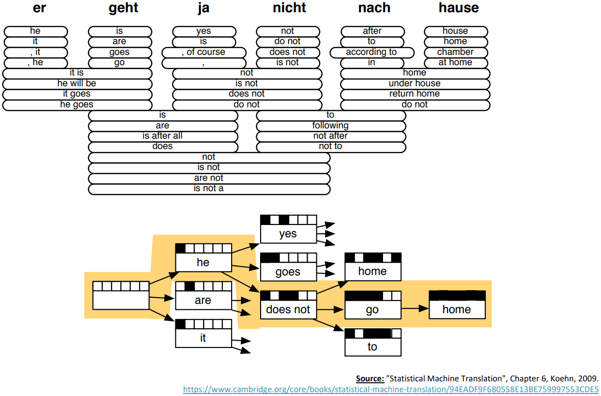
about SMT

• SMT was a huge research field
• The best systems were extremely complex
  • Hundreds of important details we haven’t mentioned here
  • Systems had many separately-designed subcomponents
  • Lots of feature engineering; need to design features to capture particular language phenomena
  • Require compiling and maintaining extra resources (like tables of equivalent phrases)
  • Lots of human effort to maintain; repeated effort for each language pair
  • Fairly successful, Google Translate launched in mid 2000s.

Neural Machine Translation (2014~)

• Neural Machine Translation (NMT) is a way to do Machine Translation with a single end-to-end neural network

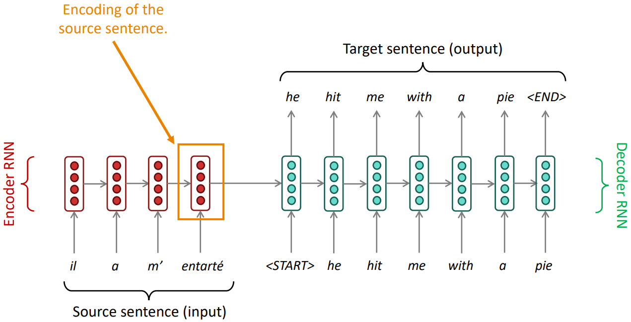
• The neural network architecture is called a sequence-to-sequence model (aka seq2seq) and it involves two RNNs

Sequence-to-sequence Model

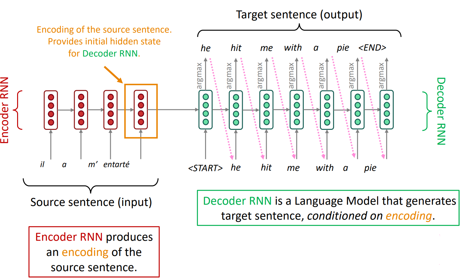
(Note: This diagram shows test time behavior: decoder output is fed in as next step’s input)

• Sequence-to-sequence is useful for more than just MT
  Many NLP tasks can be phrased as sequence-to-sequence:
  • Summarization (long text $\rightarrow$ short text)
  • Dialogue (previous utterances $\rightarrow$ next utterance)
  • Parsing (input text $\rightarrow$ output parse as sequence)
  • Code generation (natural language $\rightarrow$ Python code)
• An example of a Conditional Language Model
  • Language Model because the decoder is predicting the next word of the target sentence y
  • Conditional because its prediction are also conditioned on the source sentence x

• NMT directly calculates $P(y\vert x)$:
  $P(y|x) = P(y_1|x)P(y_2|y_1,x)P(y_3|y_1,y_2,x)\ldots P(y_T|y_1,\ldots, y_{T-1}, x)$

• Question: How to train a NMT system?

Training a Neural Machine Translation system

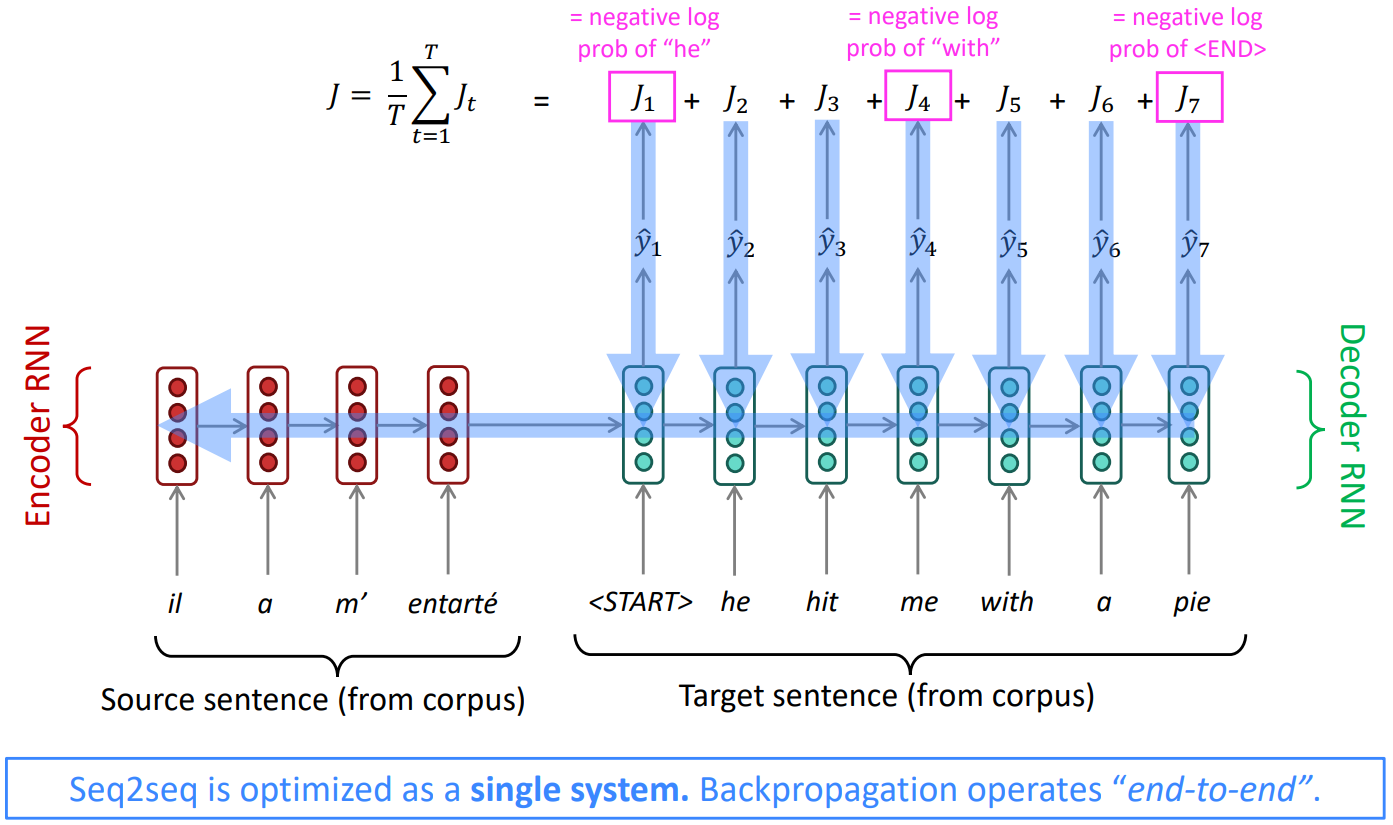
• End-to-End: update all of the parameters of the both encoder and decoder.

Multi-layer RNNs

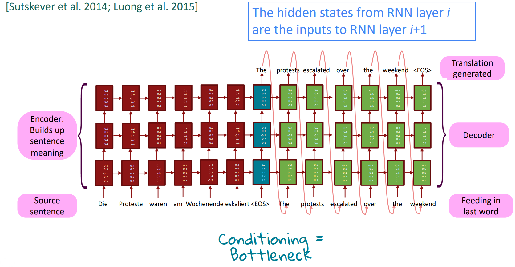
• RNNs are already “deep” on one dimension (they unroll horizontally over many timesteps), but shallow; a single layer of recurrent structure about the sentences.
• We can also make them “deep” in another dimension by applying multiple RNNs - a multi-layer RNN(or stacked RNNs). This allows the network to compute more complex representations; The lower RNNs should compute lower-level features and the higher RNNs should compute higher-level features.
• It’s not same: four LSTMs with a hidden state 500 each are more powerful than one 2000 layer LSTM (though we have the same number of parameters roughly).

Multi-layer deep encoder-decoder machine translation net

Multi-layer RNNs in practice

• High-performing RNNs are usually multi-layer (but aren’t as deep as convolutional or feed-forward networks)

• For example: In a 2017 paper, (“Massive Exploration of Neural Machine Translation Architecutres”, Britz et al.) find that for Neural Machine Translation, 2 to 4 layers is best for the encoder RNN, and 4 layers is best for the decoder RNN
  • Often 2 layers is a lot better than 1, and 3 might be a little better than 2 (rules of thumb)
  • Usually, skip-connections/dense-connections are needed to train deeper RNNs (e.g., 8 layers)
• Transformer-based networks (e.g., BERT) are usually deeper, like 12 or 24 layers having a lot of skipping-like connections.

Greedy Decoding

• Greedy decoding(take most probable word on each step) is what we saw so far; taking argmax on each step of the decoder
  • Problem: has no way to undo decisions

Exhaustive search decoding

• Ideally, we want to find a (length T) translation y that maximizes
  \(\begin{align*} P(y|x) &= P(y_1|x)P(y_2|y_1,x)P(y_3|y_1,y_2,x)\ldots P(y_T|y_1,\ldots, y_{T-1}, x) \\ &= \prod_{t=1}^T P(y_t|y_1,\ldots,y_{t-1},x) \end{align*}\)

• We could try computing all possible sequences y

  • This means that on each step t of the decoder, we’re tracking $V^t$ possible partial translations, where V is vocab size
  • This $O(V^T)$ complexity is far too expensive

Beam search decoding

• Core idea: On each step of decoder, keep track of the k most probable partial translations (which we call hypotheses)
  • k is the beam size (in practice around 5 to 10)
• A hypothesis $y_1, \ldots, y_t$ has a score which is its log probability:
  $\text{score}(y_1, \ldots, y_t) = \log P_{LM}(y_1, \ldots, y_t|x) = \sum_{i=1}^t \log P_{LM}(y_i|y_1, \ldots, y_{i-1},x)$
  • Scores are all negative, and higher is better
  • Search for high-scoring hypotheses, tracking top k on each step

• Not guaranteed to find optimal solution, but much more efficient

• Stopping criterion
  • In greedy decoding, usually we decode until the model produces an <END> token (“<START> he hit me with a pie <END>”)
  • In beam search decoding, different hypotheses may produce <END> tokens on different timesteps
    • When a hypothesis produces <END>, that hypothesis is complete.
    • Place it aside and continue exploring other hypotheses via beam search.
  • Usually continue beam search until:
    • We reach timestep T or we have at least n completed hypotheses (where T and n are some pre-defined cutoff)
• Finishing up
  • We have our list of completed hypotheses. Then how to select top one with highest score?
  • Each hypothesis $y_1,\ldots, y_t$ on our list has a score:
    \(\text{score}(y_1, \ldots, y_t) = \log P_{LM}(y_1, \ldots, y_t|x) = \sum_{i=1}^t \log P_{LM}(y_i|y_1, \ldots, y_{i-1},x)\)
  • Problem: longer hypotheses have lower scores
  • Fix: Normalize by length.
    \(\frac{1}{t}\sum_{i=1}^t \log P_{LM}(y_i|y_1, \ldots, y_{i-1},x)\)

Advantages of NMT

• Better performance:
  More fluent
  Better use of context
  Better use of phrase similarities

• A single neural network to be optimized end-to-end
  No subcomponents to be individually optimized

• Requires much less human engineering effort
  No feature engineering
  Same method for all language pairs

Disadvantages of NMT

• Less interpretable
  Hard to debug

• Difficult to control
  For example, can’t easily specify rules or guidelines for translation
  Safety concerns

How do we evaluate Machine Translation?

• BLEU (Bilingual Evaluation Understudy)
  Compares the machine-written translation to one or several human-written translation(s), and computes a similarity score based on:
  • n-gram precision (usually 1 to 4)
  • Plus a penalty for too-short system translations
• Useful but imperfect
  There are many valid ways to translate a sentence
  So a good translation can get a poor BLEU score because it has low n-gram overlap with the human translation

MT progress over time

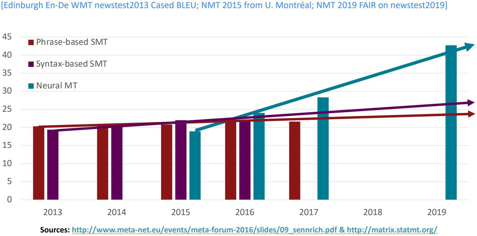
• NMT: perhaps the biggest success story of NLP Deep Learning?
  Neural Machine Translation went from a fringe research attempt in 2014 to the leading standard method in 2016
  • 2014: First seq2seq paper published
  • 2016: Google Translate switches from SMT to NMT – and by 2018 everyone has
  • SMT systems, built by hundreds of engineers over many years, outperformed by NMT systems trained by a small group of engineers in a few months
• Many difficulties remain:
  • Out-of-vocabulary words
  • Domain mismatch between train and test data
  • Maintaining context over longer text
  • Low-resource language pairs
  • Failures to accurately capture sentence meaning
  • Pronoun (or zero pronoun) resolution errors
  • Morphological agreement errors
  • Bias in training data

ATTENTION

• Information bottlenect: the last hidden state of encoder RNN needs to capture all information about the source sentence.

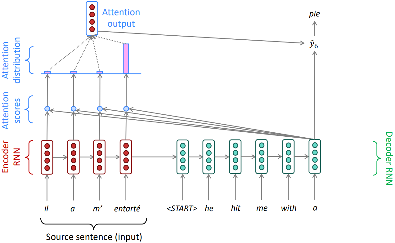
• Core idea: on each step of the decoder, use direct connection to the encoder to focus on a particular part of the source sequence

  • Each step, dot products a decoder hidden state to all encoder hidden states and get Attention scores
  • Take softmax to turn scores into Attention distribution
  • Using this distribution, take a weighted sum of the encoder hidden states to calculate Attention output
  • Concatenate with decoder hidden state, predict $\hat{y_i}$