Activation Functions

Sigmoid

• $\sigma(x)=1/(1+e^{-x})$
  • Squashes numbers to range [0,1]
  • Historically popular since they have nice interpretation as a saturating “firing rate” of a neuron.
• Problem:
  • Gradient Vanishing: Saturated neurons “kill” the gradients; If all the gradients flowing back will be zero and weights will never change.
  • Sigmoid outputs are not zero-centered and always positive, so the gradients will be always all positive or all negative. Then the gradient update would follow a zig-zag path, resulting in bad efficiency.
  • exp() is a bit compute expensive.

tanh(x)

• Squashes numbers to range [-1,1]
  zero centered
  but still kills gradients when saturated

ReLU(Rectified Linear Unit)

• \(f(x) = \mbox{max}(0,x)\)
  Does not saturate (in + region)
  Very computationally efficient
  Converges much faster than sigmoid/tanh
  but has not zero-centered output and weights will never be updated for negative x

Leaky ReLU

• \(f(x) = \mbox{max}(0.01x,x)\)
  (or parametric, PReLU: \(f(x) = \mbox{max}(\alpha x, x)\))
  Not saturate
  Computationally efficient
  Converges much faster
  will not “die”

ELU(Exponential Linear Units)

• \(f(n)= \begin{cases} x & \mbox{if }x>0 \\ \alpha(\mbox{exp}(x)-1) & \mbox{if }x\le 0\end{cases}\)
  ($\scriptstyle{\alpha = 1}$)
  All benefits of ReLU
  Closer to zero mean outputs
  Negative saturation regime compared with Leaky ReLU adds some robustness to noise
  Computation requires exp()

SELU (Scaled Exponential Linear Units)

• \(f(n)= \begin{cases} \lambda x & \mbox{if }x>0 \\ \lambda\alpha(e^x -1) & \mbox{otherwise}\end{cases}\)
  ($\scriptstyle{\alpha=1.6733, \lambda=1.0507}$)
  Scaled versionof ELU that works better for deep networks
  “Self-normalizing” property;
  Can train deep SELU networks without BatchNorm

Maxout “Neuron”

• \(\mbox{max}(w_1^T x + b_1, w_2^T x + b_2)\)
  Nonlinearity; does not have the basic form of dot product
  Generalizes ReLU and Leaky ReLU
  Linear Regime; does not saturate or die
  Complexity; Doubles the number of parameters/neuron

Swish

• \(f(x)=x\sigma(\beta x)\)
  train a neural network to generate and test out different non-linearities
  outperformed all other options for CIFAR-10 accuracy

Summary

• Use ReLU and be careful with learning rates
  Try out Leaky ReLU / Maxout / ELU / SELU to squeeze out some marginal gains
  Don’t use sigmoid or tanh

Data Preprocessing

• We may have zero-centered, normalized, decorrelated(PCA) or whitened data
• After normalization, it will be less sensitive to small changes in weights and easier to optimize
• In practice for images, centering only used.

Weight Initialization

• First idea: Small random numbers
  (gaussian with zero mean and 1e-2 standard deviation)

W = 0.01 * np.random.randn(D_in, D_out)

• It works okay for small networks, but problems with deeper networks
  All activations and gradients tend to zero and no learning proceeded.

“Xavier” Initialization

• std = 1/sqrt(D_in)
  For conv layers, $\mbox{D_in}$ is $\mbox{filter_size}^2\times \mbox{input_channels}$

W = np.random.randn(D_in, D_out) / np.sqrt(D_in)  
x = np.tanh(x.dot(W))

• Activations are nicely scaled for deeper layers
  works well especially in non-linear activation functions like sigmoid, tanh
  but cannot used in ReLU activation function; activations collapse to zero and no learning

Kaiming / MSRA Initialization

• ReLU correction: std = sqrt(2/D_in)

W = np.random.randn(D_in, D_out) * np.sqrt(2/D_in)  
x = np.maximum(0, x.dot(W))

Batch Normalization

• To make each dimension zero-mean unit-variance, apply:
  \(\hat{x}^{(k)} = \frac{x^{(k)} - E[x^{(k)}]}{\sqrt{\mbox{Var}[x^{(k)}]}}\)

• Usually inserted after Fully Connected or Convolutional layers, and before nonlinearity.

• Makes deep networks much easier to train
  Improves gradient flow
  Allows higher learning rates, faster convergence
  Networks become more robust to initialization
  Acts as regularization during training
  Zero overhead at test-time: can be fused with conv
  Behaves differently during training and testing: can have bugs

• Comparison of Normalization Layers

Transfer Learning

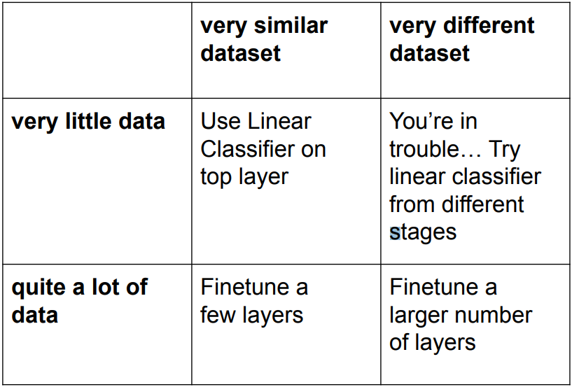
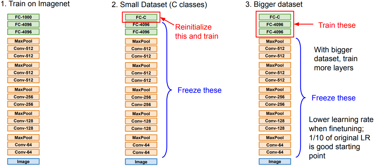
• Deep learning models are trained to capture characteristics of data, from general features at the first layer to specific features at the last layer.

• In transfer learning, we import pre-trained model and fine-tune to our cases.

• Strategies

• E.g.

• Transfer learning with CNNs is pervasive,
  for Object Detection(Fast R-CNN), Image Captioning(CNN + RNN), etc.
  but not always be necessary