What’s going on inside ConvNets?

Visualizing what models have learned

• First layer: Visualize Filters
  At the first layer, we can visualize the raw weights and see gabor-like features. While the higher layers are about the weights to the activations from the layer before, it is not very interpretable.
• Last layer: Visualize Representations(feature vector)
  • Nearest neighbors in feature space
  • Dimensionality reduction: clustering with similarity; using simple algorithm(PCA) or more complex one(t-SNE)
• Visualizing Activations:
  Yosinski et al, “Understanding Neural Networks Through Deep Visualization”, ICML DL Workshop 2014.

Understanding input pixels

• Maximally Activating Patches
  Run many images, record values of chosen channel(layer or neuron) and visualize image patches that correspond to maximal activations.
• Saliency via Occlusion: Zeiler and Fergus, “Visualizing and Understanding Convolutional Networks”, ECCV 2014.
  Mask part of the image before feeding to CNN, slide the occluder and check how much predicted probabilities change. Found that when there are multiple objects, the classification performance improved as the false class object masked.
• Which pixels matter: Saliency via Backprop
  • Visualize the data gradient
    1. foward an image
    2. set activations in layer of interest to all zero, except for a 1.0 for a neuron of interest
    3. backprop to image input
    4. squish the channels of gradients to get 1-dimensional activation map(or we can run segmentation using grabcut on this heatmap).
  • Can also find biases; to see what false classifier actually see
• Intermediate Features via (guided) backprop
  • Deconvolution-based approach:
    1. Feed image into net
    2. Pick a layer, set the gradient there to be all zero except for one 1 for some neuron of interest
    3. Backprop to image(use guided backprop to pass the positive influence; activation with positive values, using modified relu or deconvnet)
• Visualizing CNN features: Gradient Ascent (Guided) backprop: Find the part of an image that a neuron responds to.
  Gradient ascent: Generate a synthetic image that maximally activates a neuron.
  \(I^{\ast} = \mbox{argmax}_I f(I) + R(I)\); (neuron value + regularizer)
  • Optimization-based approach: freeze/fix the weights and run “image update” to find images that maximize the score of chosen class.
    Karen Simonyan, Andrea Vedaldi, Andrew Zisserman, “Deep Inside Convolutional Networks: Visualizing Image Classification Models and Saliency Maps”, Workshop at ICLR, 2014.
  • Find images that maximize some class score: \(\mbox{argmax}_I S_c(I) - \lambda {\lVert I \rVert}^2_2\)
    1. initialize image to zeros
    2. forward image to compute current scores
    3. set the gradient of the scores vector to be I, then backprop to image
    4. make a small update to the image
  • Instead of using L2 norm, we can use better regularizer(Gaussian blur image, Clip pixels with small values/gradients to 0, …)
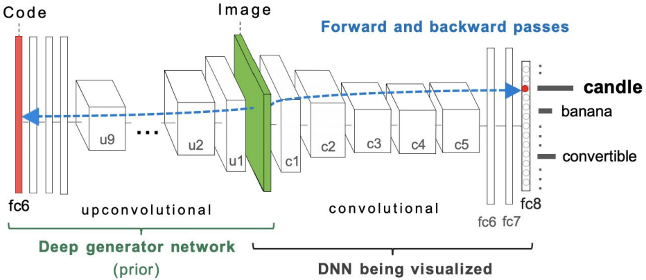
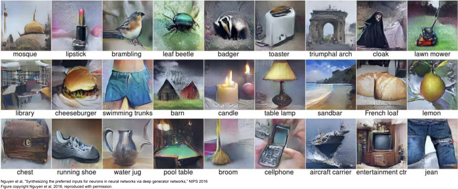
• Optimize in FC6 latent space instead of pixel space:
  
  

Adversarial perturbations

• Fooling Images / Adversarial Examples
  1. Start from an arbitrary image
  2. Pick an arbitrary class
  3. Modify the image to maximize the class
  4. Repeat until network is fooled
• Ian Goodfellow, “Explaining and Harnessing Adversarial Examples”, 2014
  Classifier is vulnerable to adversarical perturbation because of its linear nature. Check Ian Goodfellow’s lecture from 2017
• Moosavi-Dezfooli, Seyed-Mohsen, et al. “Universal adversarial perturbations”, IEEE, 2017.

Style Transfer

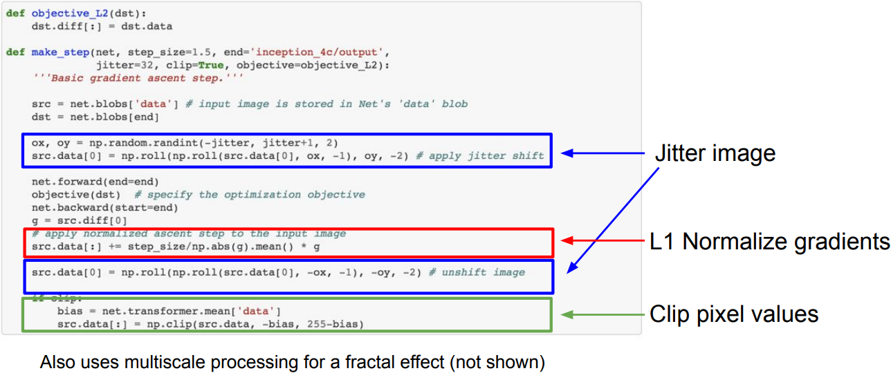
• DeepDream: Amplify existing features
  Rather than synthesizing an image to maximize a specific neuron, instead try to amplify the neuron activations at some layer in the network.
• Choose an image and a layer in a CNN; repeat:
  1. Forward: compute activations at chosen layer
  2. Set gradient of chosen layer equal to its activation
  3. Backward: Compute gradient on image
  4. Update image

• Feature Inversion
  Mahendran and Vedaldi, “Understanding Deep Image Representations by Inverting Them”, CVPR 2015
  Given a CNN feature vector for an image, find a new image that:
  • Matches the given feature vector
  • “looks natural” (image prior regularization)
    \(\begin{align*} x^{\ast} &= \underset{x\in\mathbb{R}^{H \times W \times C}}{\mbox{argmin}} l(\Phi(x), \Phi_0) + \lambda \mathcal{R}(x) \\ & \mbox{where loss } l = {\lVert \Phi(x) - \Phi_0 \rVert}^2 \end{align*}\)

• Texture Synthesis: Nearest Neighbor
  Given a sample patch of some texture, generate a bigger image of the same texture
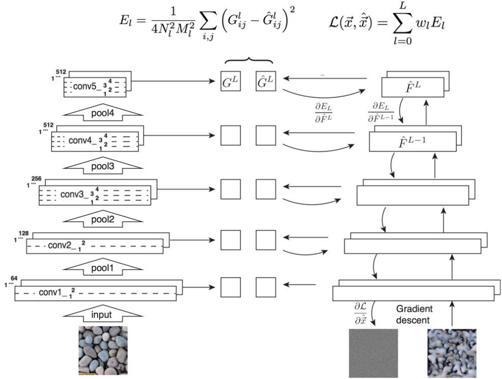
  Generate pixels one at a time in scanline order; form neighborhood of already generated pixels and copy nearest neighbor from input

• Neural Texture Synthesis: Gram Matrix
  a pair-wise statistics; interpret given CxHxW features as HxW grid of C-dimensional vectors. By computing outer product and sum up for all spacial locations($G=V^T V$), it gives CxC matrix measuring co-occurrence.
  1. Pretrain a CNN on ImageNet (VGG-19)
  2. Run input texture forward through CNN, record activations on every layer
  3. At each layer compute the Gram matrix
  4. Initialize generated image from random noise
  5. Pass generated image through CNN, compute Gram matrix on each layer
  6. Compute loss: weighted sum of L2 distance between Gram matrices
  7. Backprop to get gradient on image
  8. Make gradient step on image
  9. GOTO 5
• Neural Style Transfer: Feature + Gram Reconstruction
  1. Extract content targets (ConvNet activations of all layers for the given image)
  2. Extract style targets (Gram matrices of ConvNet activations of all layers)
  3. Optimize over image to have:
     • The content of the content image(activations match content)
     • The style of the stlye image(Gram matrices of activations match style)
       
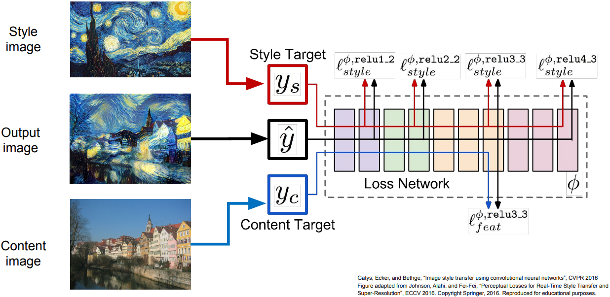
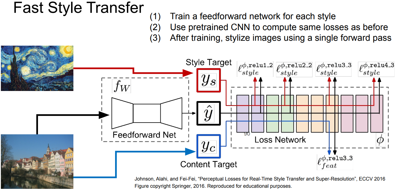
     • Problem: requires many forward, backward passes; VGG is very slow
     • Solution: Train another neural network; Fast Style Transfer
• Fast Style Transfer