The Simple RNN Language Model

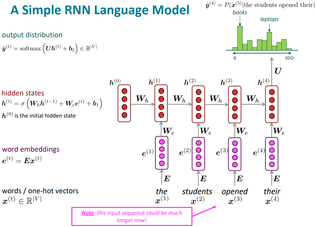
Training an RNN Language Model

• Get a big corpus of text which is a sequence of words $x^{(1)}, \ldots, x^{(T)}$
• Feed into RNN-LM; compute output distribution $\hat{y}^{(t)}$ for every step $t$.
  i.e., predict probability distribution of every word, given words so far

• Loss function on step is cross-entropy(negative log-likelihood) between predicted probability distribution $\hat{y}^{(t)}$, and the true next word $y^{(t)}$(one-hot for $x^{(t+1)}$):
  \(\begin{align*} J^{(t)}(\theta) = CE(y^{(t)}, \hat{y}^{(t)}) = -\sum_{w\in V} y_w^{(t)} \log \hat{y}_w^{(t)} = -\log \hat{y}_{x_{t+1}}^{(t)} \end{align*}\)

• Average this to get overall loss for entire training set:
  \(\begin{align*} J(\theta) = \frac{1}{T}\sum_{t=1}^T J^{(t)}(\theta) = \frac{1}{T}\sum_{t=1}^T -\log \hat{y}_{x_{t+1}}^{(t)} \end{align*}\)

• “Teacher forcing” algorithm:
  At each step, reset to what was actually in the corpus and not reuse what the model have suggested.

• However: Computing loss and gradients across entire corpus $x^{(1)}, \ldots, x^{(T)}$ is too expensive
  In pratice, consider $x^{(1)}, \ldots, x^{(T)}$ as a sentence or a document

• Recall: Stochastic Gradient Descent allows us to compute loss and gradients for small chunk of data, and update.
  Compute loss $J(\theta)$ for a sentence (actually, a batch of sentences), compute gradients and update weights. Repeat.

Training the parameters RNNs: Backpropagation for RNNs

• Question: What’s the derivative of $J^{(t)}(\theta)$ w.r.t. the repeated weight matrix $W_h$?

• Answer: sum of the gradient w.r.t. each time it appears
  \(\begin{align*} \frac{\partial J^{(t)}}{\partial W_h} = \sum_{i=1}^t \left. \frac{\partial J^{(t)}}{\partial W_h} \right|_{(i)} \end{align*}\)

• Backpropagation for RNNs: Proof sketch

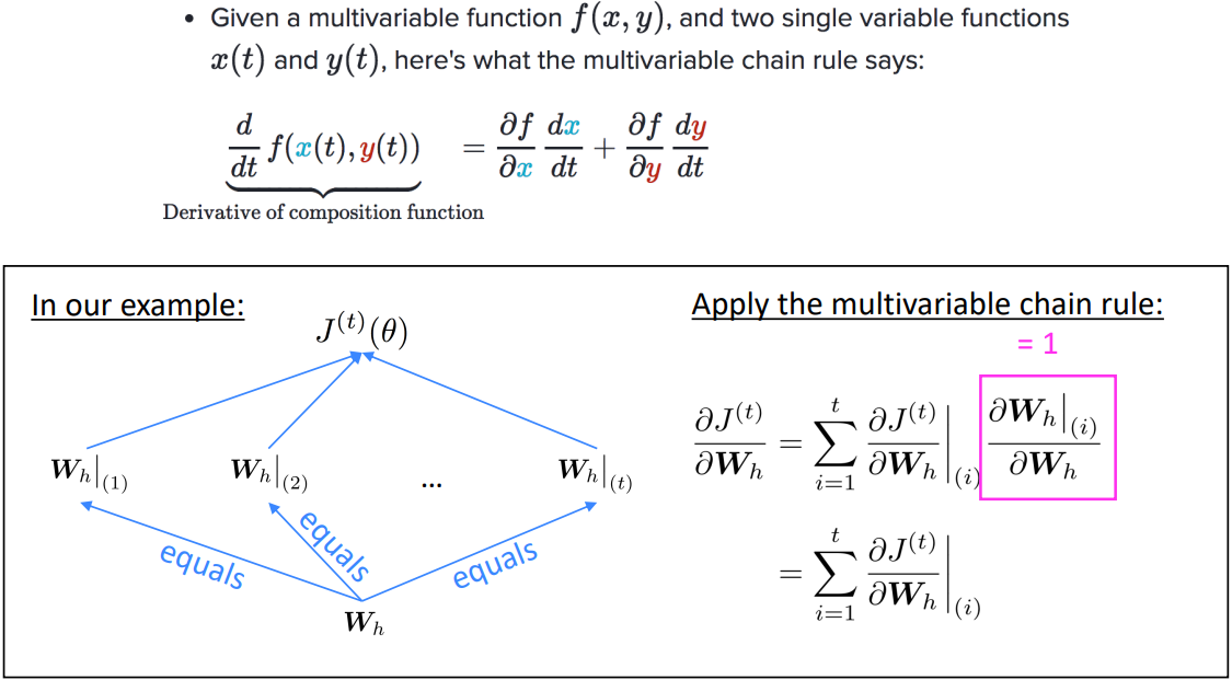
• How to calculate:
  Backpropagate over timesteps $i=t,\ldots,0$, summing gradients as you go.
  “Backpropagation through time, [Werbos, P.G., 1988, Neural Networks 1, and others]”

Generating text with a RNN Language Model

• Like a n-gram Language Model, use an RNN Language Model to generate text by repeated sampling. Sampled output becomes next step’s input.

• You can train an RNN-LM on any kind of text, then generate text in that style.

Evaluating Language Models

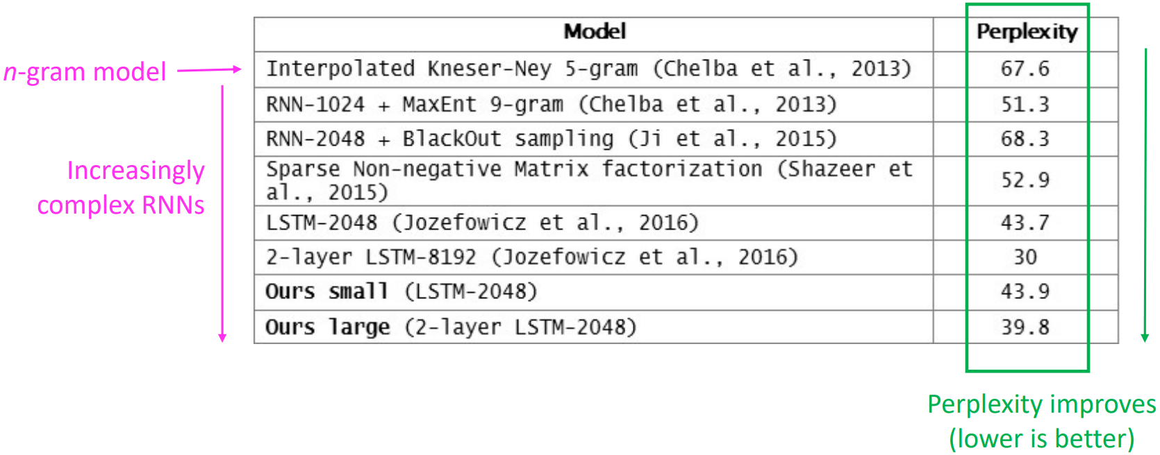
• The standard evaluation metric for Language Model is perlexity; a geometric mean of the inverse probabilities.

• This is equal to the exponential of the cross-entropy loss $J(\theta)$:
  \(\begin{align*} = \prod_{t=1}^T \left( \frac{1}{\hat{y}_{x_{t+1}}^{(t)}}\right)^{1/T} = \exp \left( \frac{1}{T}\sum_{t=1}^T -\log \hat{y}_{x_{t+1}}^{(t)} \right) = \exp(J(\theta)) \end{align*}\)
  $\rightarrow$ Lower perplexity is better

• RNNs have greatly improved perplexity

Why should we care about Language Modeling?

• Language Modeling is a benchmark task that helps us measure our progress on understanding language

• Language Modeling is a subcomponent of many NLP tasks, especially those involving generating text or estimating the probability of text:

  • Predictive typing
  • Speech recognition
  • Handwriting recognition
  • Spelling/grammar correction
  • Authorship identification
  • Machine translation
  • Summarization
  • Dialogue
  • etc.

Recap

• Language Model: A system that predicts the next word

• Recurrent Neural Network: A family of neural networks that:
  • Take sequential input of any length
  • Apply the same weights on each step
  • Can optionally produce output on each step
• Recurrent Neural Network $\ne$ Language Model
  shown that RNNs are a great way to build a LM, but RNNs are useful for much more

Other RNN uses

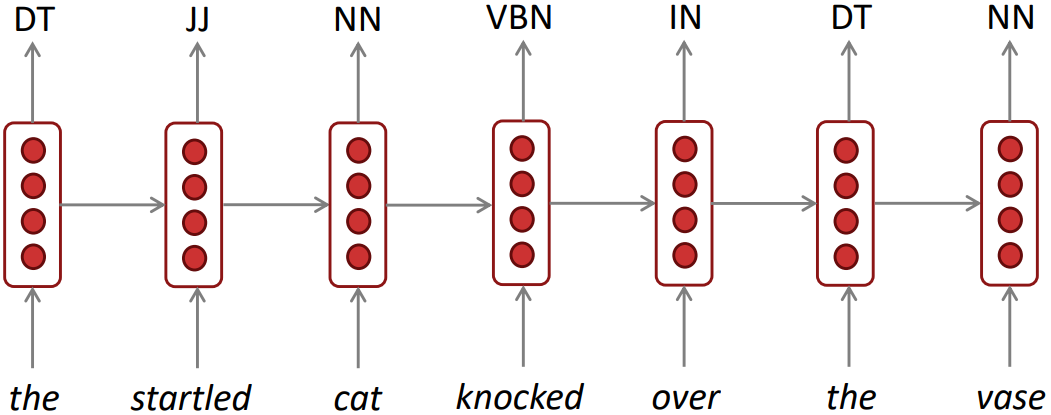
• Sequence tagging: e.g., part-of-speech tagging, named entity recognition
  

• Sentence classification: e.g., sentiment classification
  
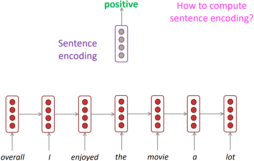
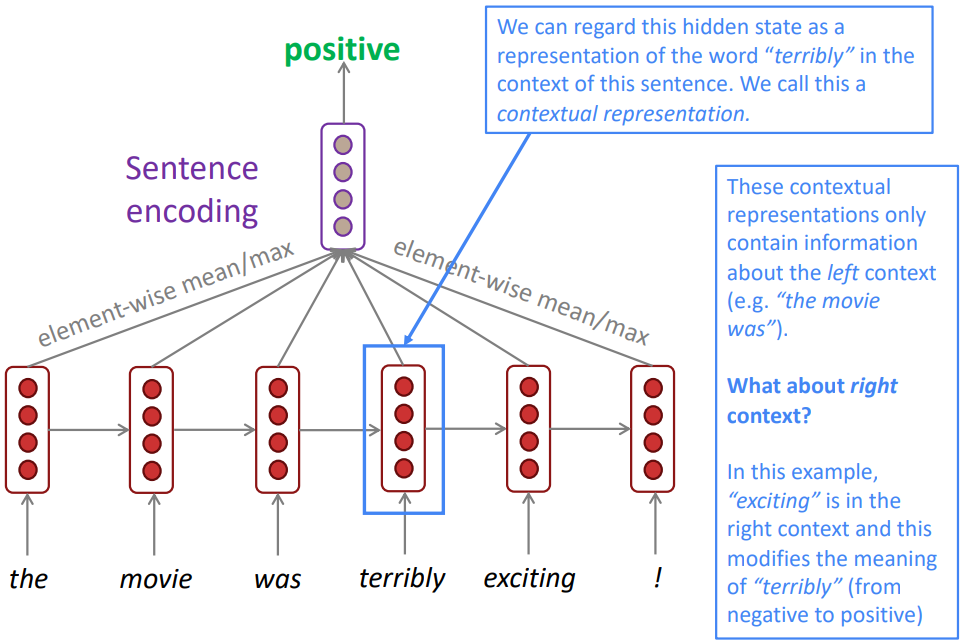
  1. Basic way: Use the final hidden state. After running RNN(or LSTM), the final hidden state was encoded the whole sentence and treat it as the whole meaning of the sentence. Then put an extra classifier layer.
  2. Usually better:
     Take element-wise max or mean of all hidden states to more symmetrically encode the hidden state over each time step.

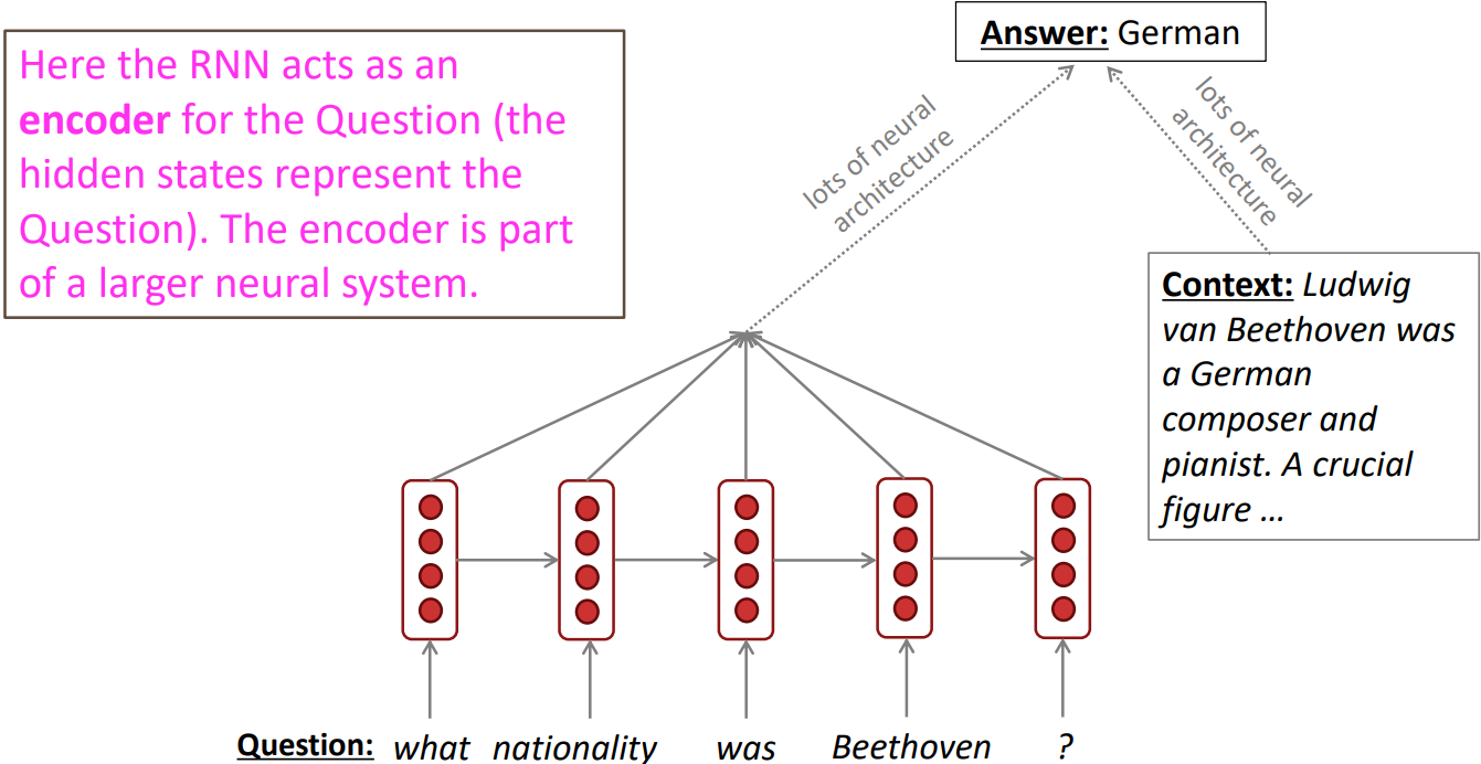
• Language encoder module: e.g., question answering, machine translation, many other tasks
  

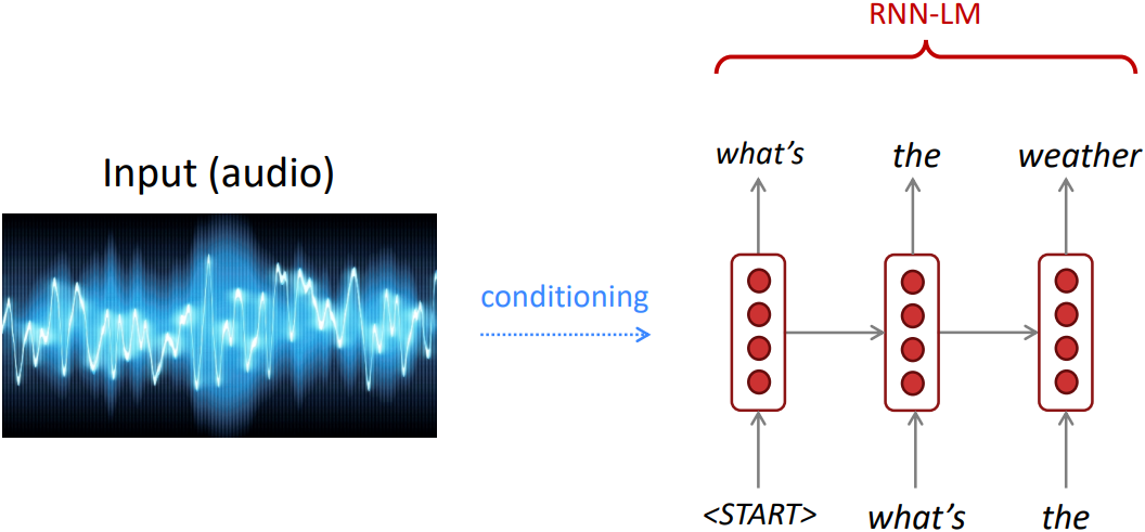
• Generate text: e.g., speech recognition, machine translation, summarization
  

Problems with Vanishing and Exploding Gradients

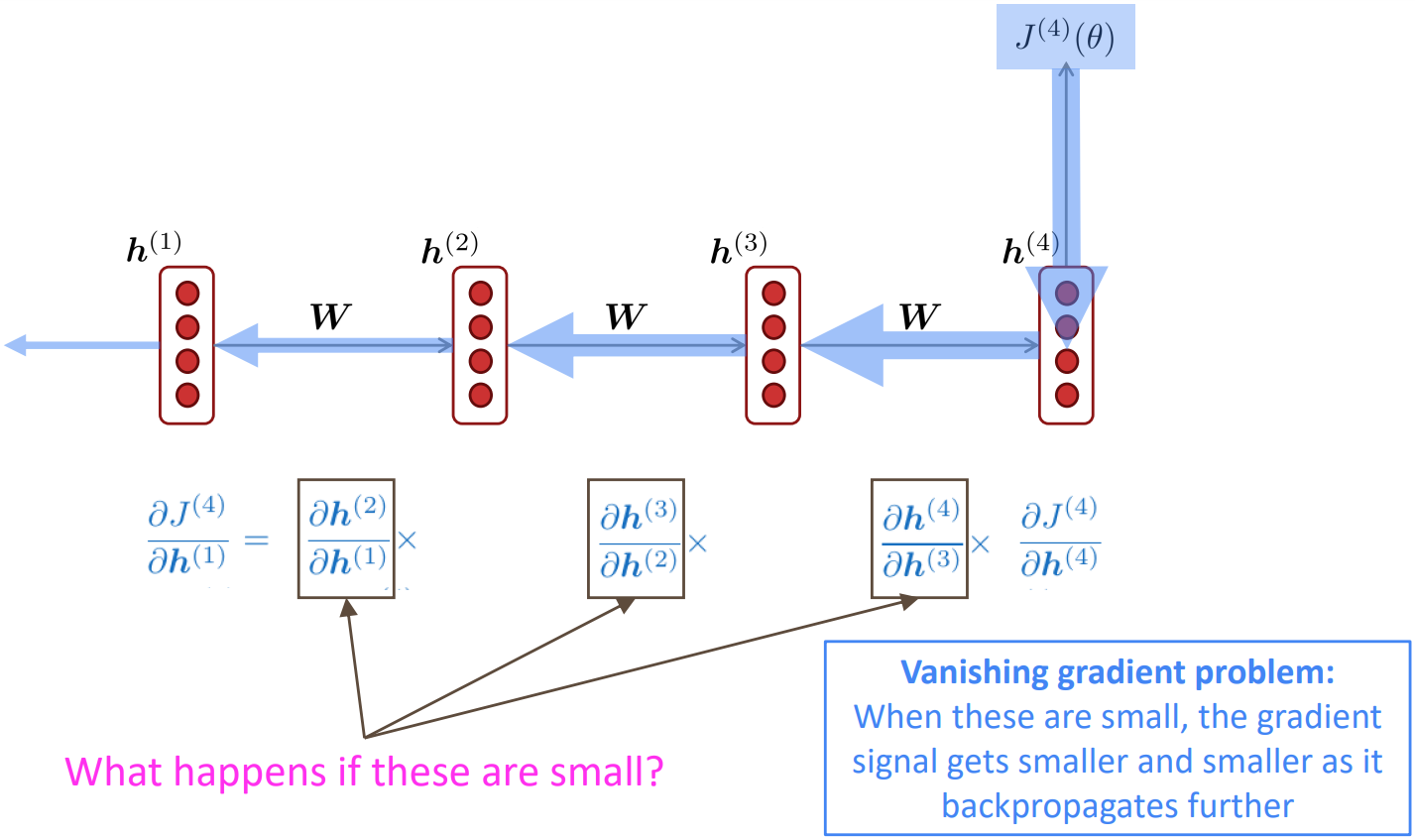
Vanishing gradient: Proof sketch (linear case)

• Recall:
  $\hat{h}^{(t)} = \sigma(W_h h^{(t-1)} + W_x x^{(t)} + b_1)$
• What if $\sigma(x) = x$?
  \(\begin{align*} \frac{\partial h^{(t)}}{\partial h^{(t-1)}} &= \text{diag} \left( \sigma^\prime \left( W_h h^{(t-1)} + W_x x^{(t)} + b_1 \right) \right) W_h &&(\text{chain rule}) \\ &= I\ W_h = W_h \end{align*}\)
• Consider the gradient of the loss $J^{(i)}(\theta)$ on step $i$, w.r.t. the hidden state $h^{(j)}$ one some previous step $j$. Let $l = i - j$
  \(\begin{align*} \frac{\partial J^{(i)}(\theta)}{\partial h^{(j)}} &= \frac{\partial J^{(i)}(\theta)}{\partial h^{(i)}} \prod_{j < t \le i}\frac{\partial h^{(t)}}{\partial h^{(t-1)}} &&(\text{chain rule}) \\ &= \frac{\partial J^{(i)}(\theta)}{\partial h^{(i)}} \prod_{j < t \le i} W_h = \frac{\partial J^{(i)}(\theta)}{\partial h^{(i)}} W_h^l &&(\text{value of } \frac{\partial h^{(t)}}{\partial h^{(t-1)}}) \end{align*}\)
  $\rightarrow$ If $W_h$ is “small”, then $W_h^l$ gets exponentially problematic as $l$ becomes large

• Consider if the eigenvalues of $W_h$ are all less than 1(sufficient but not necessary):
  $\lambda_1, \lambda_2, \ldots, \lambda_n < 1$
  $q_1, q_2, \ldots, q_n$ (eigenvectors)
  Rewrite using the eigenvectors of $W_h$ as a basis:
  \(\begin{align*} \frac{\partial J^{(i)}(\theta)}{\partial h^{(i)}} = \sum_{i=1}^n c_i \lambda_i^l q_i \approx 0 \end{align*}\) (for large $l$)
  $\therefore \lambda_i^l$ approaches 0 as $l$ grows, gradient vanishes

• Choosing nonlinear activations $\sigma$
  Pretty much the same thing, except the proof requires $\lambda_i < \gamma$ for some $\gamma$ dependdent on dimensionality and $\sigma$

Why is vanishing gradient a problem?

• Gradient signal from far away is lost because it’s much smaller than gradient signal from close-by. So, model weights are updated only with respect to near effects, not long-term effects.

Effect of vanishing gradient on RNN-LM

• LM task:

  “When she tried to print her tickets, she found that the printer was out of toner. She went to the stationery store to buy more toner. It was very overpriced. After installing the toner into the printer, she finally printed her [target]”

• To learn from this training example, the RNN-LM needs to model the dependency between “tickets” on the 7th step and the target word “tickets” at the end
  But if gradient is small, the model can’t learn this dependency and the model is unable to predict similar long-distance dependencies at test time

Why is exploding gradient a problem?

• If the gradient becomes too big, then the SGD update step becomes too big:
  This can cause bad updates: we take too large a step and reach a weird and bad parameter configuration (with large loss)
• In the worst case, this will result in Inf or NaN in your network
  (then you have to restart training from an earlier checkpoint)

Gradient clipping: solution for exploding gradient

• If the norm of the gradient is greater than some threshold, scale it down before applying SGD update

• Intuition: take a step in the same direction, but a smaller step

• In practice, remembering to clip gradients is important, but exploding gradients are an easy problem to solve

How to fix the vanishing gradient problem?

• The main problem is that it’s too difficult for the RNN to learn to preserve information over many timesteps

• In a vanilla RNN, the hidden state is constantly being rewritten
  $h^{(t)} = \sigma \left( W_h h^{(t-1)} + W_x x^{(t)} + b \right)$
  $\rightarrow$ How about a RNN with separate memory?

Long Short-Term Memory RNNs (LSTMs)

• Proposed by “Long short-term memory”, Hochreiter and Schmidhuber, 1997, but really a crucial part of the modern LSTM is from “Learning to Forgt: Continual Prediction with LSTM”, Gers et al., 2000.

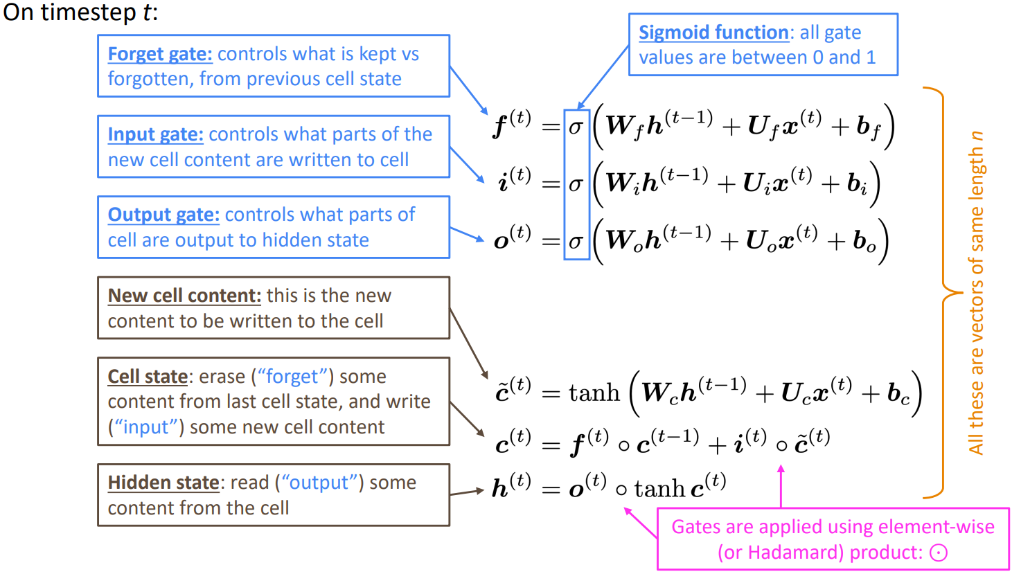
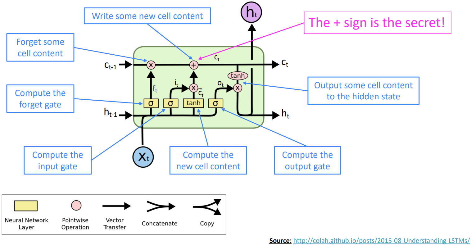
• On step $t$, there is a hidden state $h^{(t)}$ and a cell state $c^{(t)}$
  • Both are vectors length $n$
  • The cell stores long-term information
  • The LSTM can read, erase, and write information from the cell
    The cell becomes conceptually rather like RAM in a computer
• The selection of which information is erased/written/read is controlled by three corresponding gates
  • The gates are also vectors length $n$
  • On each timestep, each element of the gates can be open (1), closed (0), or somewhere in-between
  • The gates are dynamic: their value is computed based on the current context
• With a sequence of inputs $x^{(t)}$, compute a sequence of hidden states $h^{(t)}$ and cell states $c^{(t)}$.

How does LSTM solve vanishing gradients?

• The LSTM architecture makes it easier for the RNN to preserve information over many timesteps
  • e.g., if the forget gate is set to 1 for a cell dimension and the input gate set to 0, then the information of that cell is preserved indefinitely.
  • In practice, you get about 100 timesteps rather than about 7 of effective memory.
• LSTM doesn’t guarantee that there is no vanishing/exploding gradient, but it does provide an easier way for the model to learn long-distance dependencies

  LSTM: real-world success

• In 2013–2015, LSTMs started achieving state-of-the-art results
  • Successful tasks include handwriting recognition, speech recognition, machine translation, parsing, and image captioning, as well as language models
  • LSTMs became the dominant approach for most NLP tasks
• Now (2021), other approaches (e.g., Transformers) have become dominant for many tasks
  • For example, in WMT (a Machine Translation conference + competition):
    In WMT 2016, the summary report contains “RNN” 44 times
    In WMT 2019, “RNN” 7 times, “Transformer” 105 times

Is vanishing/exploding gradient just a RNN problem?

• It can be a problem for all neural architectures (including feed-forward and convolutional), especially very deep ones.
  Due to chain rule / choice of nonlinearity function, gradient can become vanishingly small as it backpropagates. Thus, lower layers are learned very slowly (hard to train)

• Solution: lots of new deep feedforward/convolutional architectures that add more direct connections (thus allowing the gradient to flow)

• For example:
  • Resnet, “Deep Residual Learning for Image Recognition”, He et al, 2015.
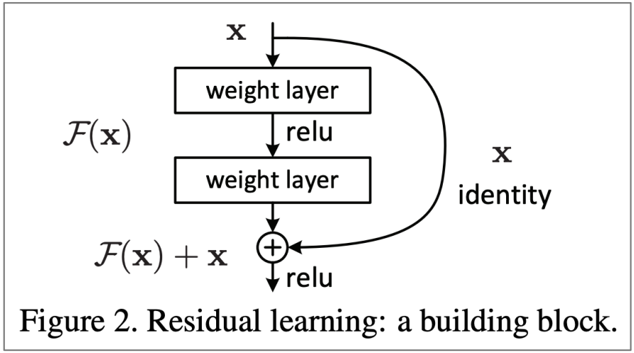
    Also known as skip-connects, the identity connection preserves information by default and makes deep networks much easier to train.
  • Densenet, “Densely Connected Convolutional Networks”, Huang et al, 2017.
    
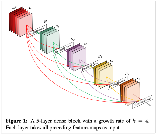
    Dense connections that directly connect each layer to all future layers
  • HighwayNet, “Highway Networks”, Srivastava et al, 2015.
    
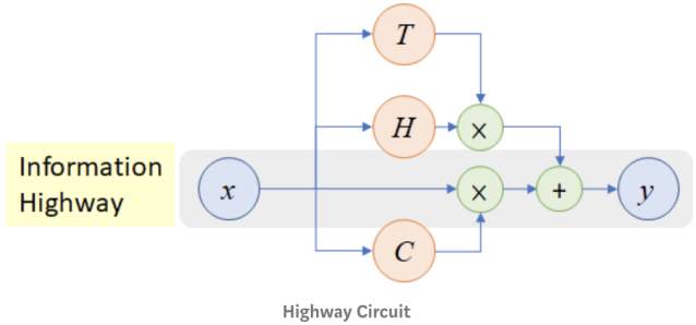
    Similar to residual connections, but controlled by a dynamic gate.
• Conclusion: Though vanishing/exploding gradients are a general problem, RNNs are particularly unstable due to the repeated multiplication by the same weight matrix (Bengio et al, 1994)

Bidirectional and Multi-layer RNNs: motivation

• Example: Sentiment Classification task

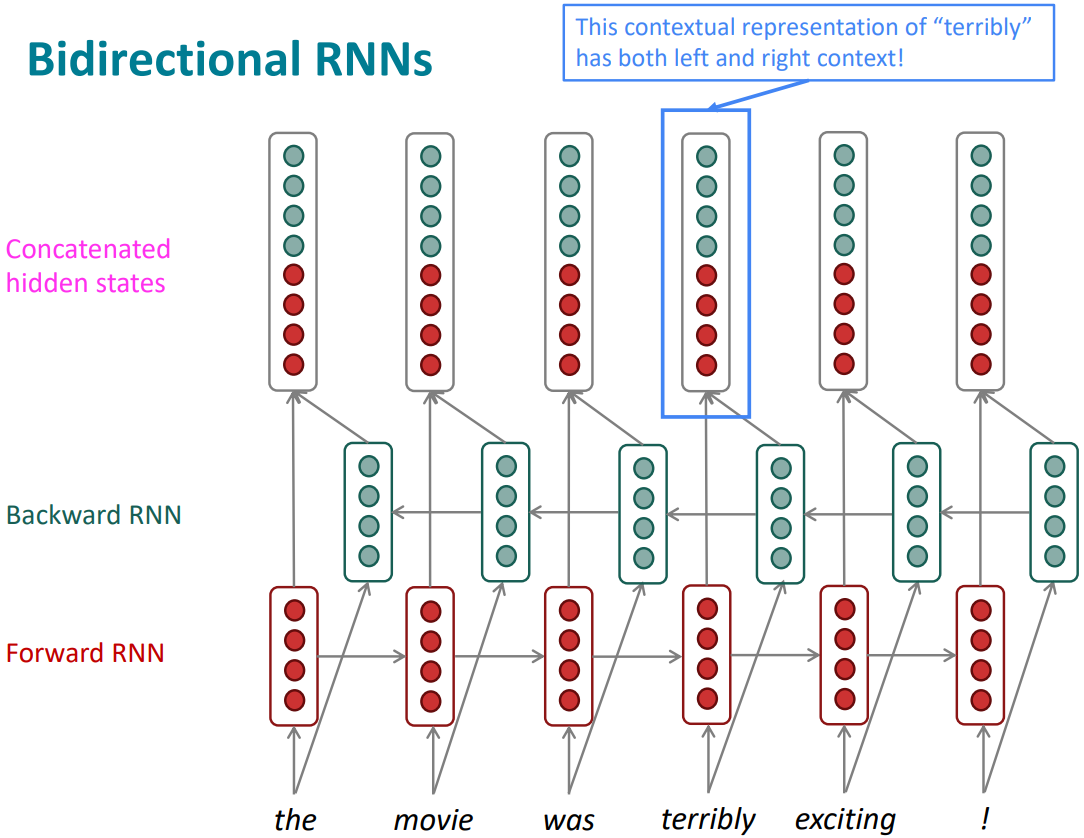
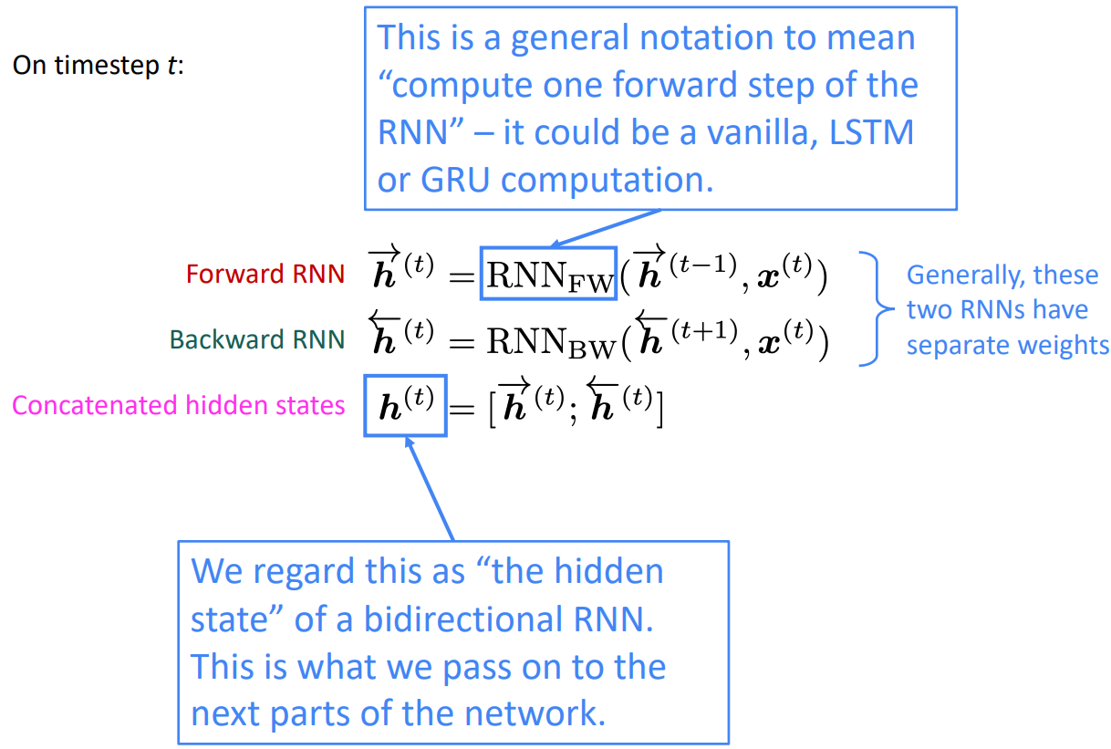
• Note: bidirectional RNNs are only applicable if you have access to the entire input sequence
  They are not applicable to Language Modeling, because in LM you only have left context available.

• If you do have entire input sequence(e.g., any kind of encoding), bidirectionality is powerful (you should use it by default).

• For example, BERT (Bidirectional Encoder Representations from Transformers) is a powerful pretrained contextual representation system built on bidirectionality.