Supervised vs. Unsupervised

• Supervised Learning:
  Data: $(x,y)$; y is label
  Goal: Learn a function to map $x\rightarrow y$

• Unsupervised Learning:
  Data: x; no labels
  Goal: Learn some underlying hidden structure of the data

Generative Modeling

Given training data, generate new samples from same distribution

• Objectives:
  1. Learn $p_{\scriptstyle\text{model}}(x)$ that approximates $p_{\scriptstyle\text{data}}(x)$
  2. Sampling new x from $p_{\scriptstyle\text{model}}(x)$
• Formulate as density estimation problems:
  • Explicit density estimation: explicitly define and solve for $p_{\scriptstyle\text{model}}(x)$.
  • Implicit density estimation: learn model that can sample from $p_{\scriptstyle\text{model}}(x)$ without explicitly defining it.
• Why Generative Models?
  Realistic samples for artwork, super-resolution, colorization, etc.
  Learn useful features for downstream tasks such as classification.
  Getting insights from high-dimensional data (physics, medical imaging, etc.)
  Modeling physical world for simulation and planning (robotics and reinforcement learning applications)
  …

PixelRNN and PixelCNN; a brief overview

• Fully visible belief network (FVBN)
  is an explicit density model, defines tractable density function using chain rule to decompose the likelihood of an image x into product of 1-d distributions:
  
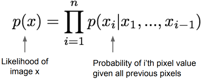
  Then maximize likelihood of training data. It is a complex distribution over pixel values, express using a neural network.

PixelRNN, van der Oord et al., 2016

• Generate image pixels starting from corner, dependency on previous pixels modeled using an RNN(LSTM).
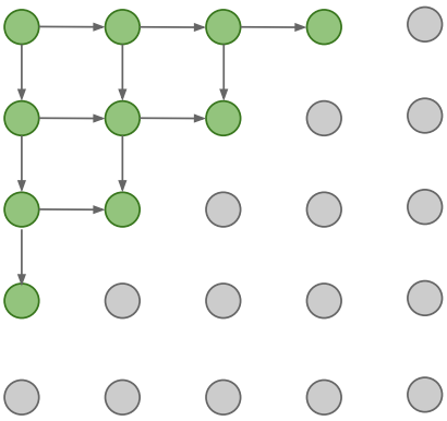
  Drawback: sequential generation is slow in both training and inference

PixelCNN, van der Oord et al., 2016

• Generate image pixels starting from corner, ependency on previous pixels modeled using a CNN over context region(masked convolution)
  
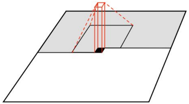
  Training is faster than PixelRNN: it can parallelize convolutions since context region values known from training images.
  Generation is still slow: for a 32x32 image, we need to do forward passes of the network 1024 times for a single image.

• Improving PixelCNN performance
  Gated convolutional layers, Short-cut connections, Discretized logistic loss, Multi-scale, Training tricks, etc.
  See also PixelCNN++, Salimans et al., 2017

Summary

• Pros:
  Can explicitly compute likelihood p(x)
  Easy to optimize
  Good samples
• Cons:
  Sequential generation is slow

Variational Autoencoder(VAE)

• VAE is an explicit density model, defines intractable(approximate) density function with latent z:
  $p_\theta(x) = \int p_\theta(z)p_\theta(x|z)\, dz$
  No dependencies among pixels, can generate all pixels at the same time. But cannot optimize directly, derive and optimize lower bound on likelihood instead

Background: Autoencoders

• Unsupervised approach for learning a lower-dimensional feature representation from unlabeled training data
  
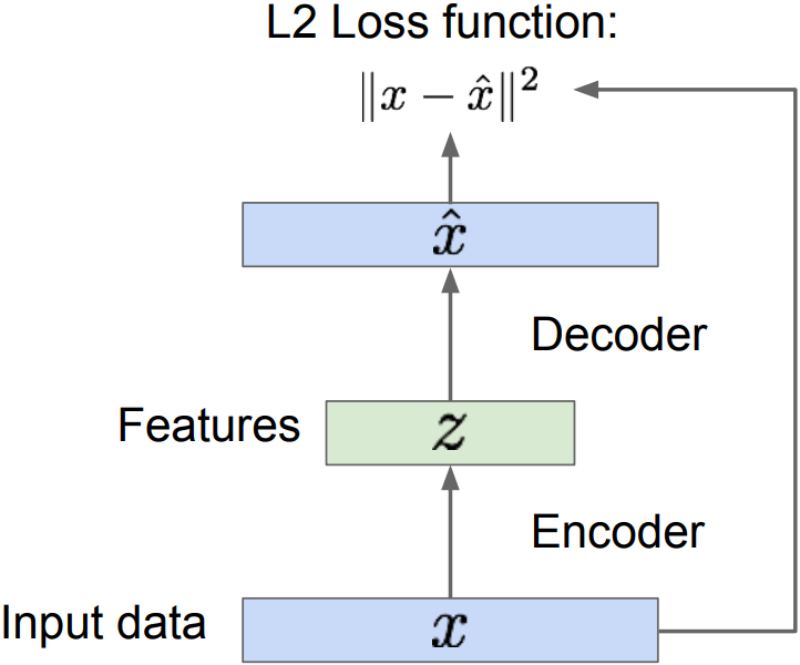
  • z usually smaller than x: with dimensionality reduction to capture meaningful factors of variation in data. Train such that features can be used to reconstruct original data($\hat{x}$)
  • “Autoencoding”; encoding input itself(L2 loss)
  • After training, throw away decoder and adjust to the final task

• Encoder can be used to initialize a supervised model; Transfer from large, unlabeled dataset(Autoencoder) to small, labeled dataset and fine-tune; train for final task.
  

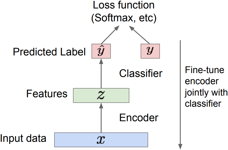
• But we can’t generate new images from an autoencoder because we don’t know the space of z. $\rightarrow$ Variational Autoencoders for a generative model.

Variational Autoencoders: Probabilistic spin on autoencoders

• Assume training data \(\left\{ x^{(i)}\right\} _{i=1}^N\) is generated from the distribution of unobserved (latent) representation z
• Intuition from autoencoders: x is an image, z is latent factors used to generate x: attributes, orientation, etc.

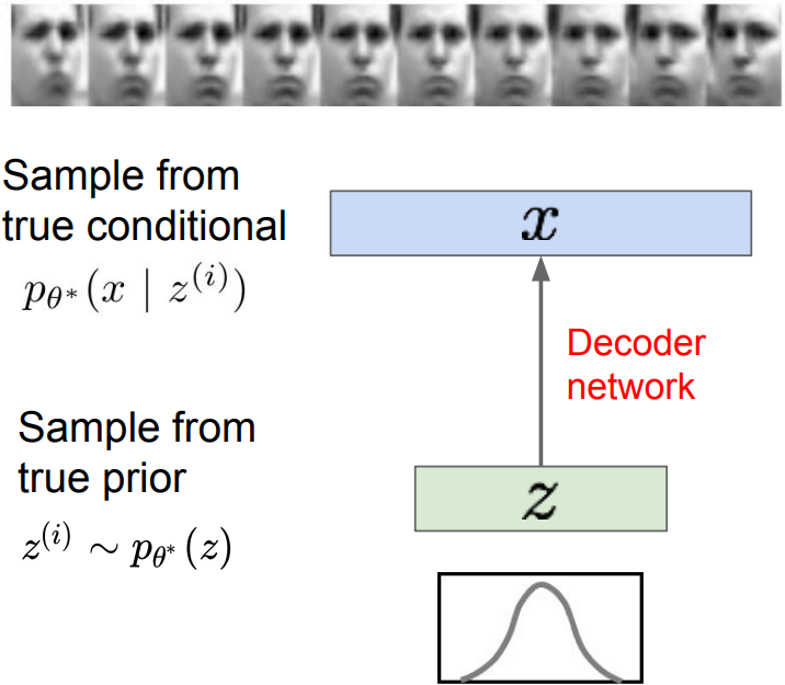
• We want to estimate the true parameters $\theta^*$ of this generative model given training data x.
• Model representation:
  • p(z): Choose prior to be simple, e.g. Gaussian.
  • z: Reasonable for latent attributes, e.g. pose, how much smile.
  • p(x|z): Generating images, conditional probability is complex
    $\rightarrow$ represent with neural network
  • $p_\theta(x)$: Learn model parameters to maximize likelihood of training data

Variational Autoencoders: Intractability

• Data likelihood:
  $p_\theta(x) = \int p_\theta(z)p_\theta(x|z)\, dz$
  where $p_\theta(z)$ is a Simple Gaussian prior and $p_\theta(x|z)$ is a decoder neural network, it is intractable to compute p(x|z) for every z.
  while Monte Carlo estimation-$\log p(x) \approx \log\frac{1}{k}\sum_{i=1}^k p(x|z^{(i)})$, where $z^{(i)}\sim p(z)$- is too high variance.
• divided by intractable $p_\theta(x)$, Posterior density also intractable:
  $p_\theta(z|x) = p_\theta(x|z)p_\theta(z)/p_\theta(x)$
• Solution:
  In addition to modeling $p_\theta(x|z)$, learn $q_\phi(z|x)$ that approximates the true posterior $p_\theta(z|x)$. $q_\phi$, approximate posterior allows us to derive a lower bound on the data likelihood that is tractable, which can be optimized.
  Variational inference is to approximate the unknown posterior distribution from only the observed data x

\[\begin{align*} \log p_\theta(x^{(i)}) &= \mathbf{E}_{z~q_\phi(z|x^{(i)})}\left[ \log p_\theta(x^{(i)}) \right] \quad \textit(p_\theta(x^{(i)})\ does\ not\ depend\ on\ z) \\ &= \mathbf{E}_z \left[ \log\frac{p_\theta(x^{(i)}|z)p_\theta(z)}{p_\theta(z|x^{(i)})} \right] \quad \textit(Bayes'\ Rule) \\ &= \mathbf{E}_z \left[ \log\frac{p_\theta(x^{(i)}|z)p_\theta(z)}{p_\theta(z|x^{(i)})} \frac{q_\phi(z|x^{(i)})}{q_\phi(z|x^{(i)})} \right] \quad \textit(Multiply\ by\ constant)\\ &= \mathbf{E}_z \left[\log p_\theta(x^{(i)}|z) \right] - \mathbf{E}_z \left[ \log\frac{q_\phi(z|x^{(i)})}{p_\theta(z)}\right] + \mathbf{E}_z \left[ \log\frac{q_\phi(z|x^{(i)})}{p_\theta(z|x^{(i)})}\right] \quad \textit(Logarithms) \\ &= \mathbf{E}_z \left[\log p_\theta(x^{(i)}|z) \right] - D_{KL}(q_\phi(z|x^{(i)})|p_\theta(z)) + D_{KL}(q_\phi(z|x^{(i)})|p_\theta(z|x^{(i)})) \end{align*}\]

• With taking expectation with respect to z(using encoder network) let us write nice KL terms;
  • \(\mathbf{E}_z \left[\log p_\theta(x^{(i)}\vert z) \right]\): Decoder network gives $p_\theta(x\vert z)$, can compute estimate of this term through sampling(need some trick to differentiate through sampling). It reconstruct the input data.
  • \(D_{KL}(q_\phi(z\vert x^{(i)})\vert p_\theta(z))\): KL term between Gaussian for encoder and z prior has nice closed-form solution. Encoder makes approximate posterior distribution close to prior.
  • \(D_{KL}(q_\phi(z\vert x^{(i)})\vert p_\theta(z\vert x^{(i)}))\): is intractable, we can’t compute this term; but we know KL divergence always greater than 0.

• To maximize the data likelihood, we can rewrite
  \(\begin{align*} \log p_\theta (x^{(i)}) &= \mathbf{E}_z \left[ \log p _\theta (x^{(i)}\vert z) \right] - D_{KL}(q_\phi (z\vert x^{(i)})\vert p_\theta (z)) + D_{KL}(q_\phi (z\vert x^{(i)})\vert p_\theta (z\vert x^{(i)})) \\ &= \mathcal{L}(x^{(i)},\theta ,\phi ) + (C\ge 0) \end{align*}\)

• \(\mathcal{L}(x^{(i)},\theta,\phi)\): Decoder - Encoder
  Tractable lower bound which we can take gradient of and optimize. Maximizing this evidence lower bound(ELBO), we can maximize $\log p_\theta(x)$. Later, we take minus on this term for the loss function of a neural network.

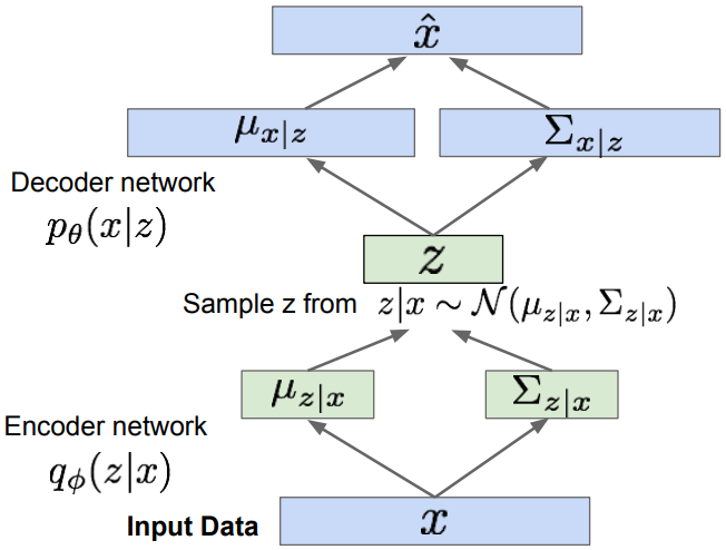
• Encoder part; \(D_{KL}(q_\phi(z\vert x^{(i)})\vert p_\theta(z))\)
  We choose q(z) as a Gaussian distribution, $q(z\vert x) = N(\mu_{z\vert x}, \Sigma_{z\vert x})$. Computing the KL divergence, \(D_{KL}(N(\mu_{z\vert x}, \Sigma_{z\vert x}))\vert N(0,I))\), having analytical solution.
• Reparameterization trick z:
  to make sampling differentiable, input sample $\epsilon\sim N(0,I)$ to the graph $z = \mu_{z\vert x} + \epsilon\sigma_{z\vert x}$; where $\mu, \sigma$ are the part of computation graph.
• Decoder part;
  Maximize likelihood of original input being reconstructed, $\hat{x}-x$.
• For every minibatch of input data, compute $\mathcal{L}$ graph forward pass and backprop.

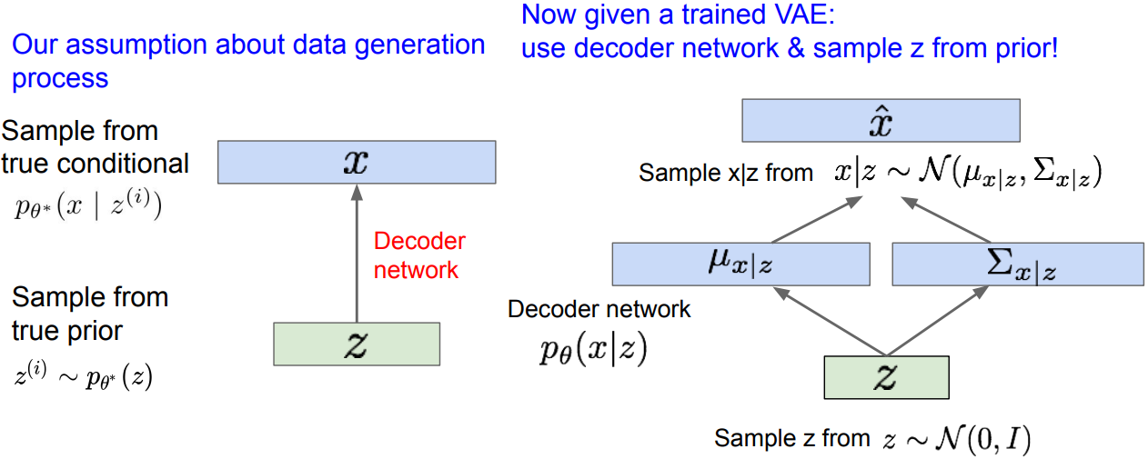
Variational Autoencoders: Generating Data

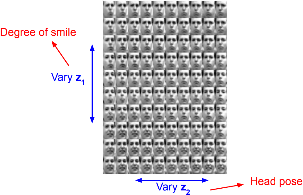
• Diagonal prior on z for independent latent variables
• Different dimensions of z encode interpretable factors of variation;
  Also good feature representation taht can be computed using $q_\phi(z\vert x)$.

Summary

• Probabilistic spin to traditional autoencoders, allows generating data

• Defines an intractable density; derive and optimize a (variational) lower bound

• Pros:
  Principled approach to generative models
  Interpretable latent space
  Allows inference of $q(z\vert x)$, can be useful feature representation for other tasks - Cons:
  Maximizes lower bound of likelihood: not as good evaluation as tractable model
  Samples mean; blurrier and lower quality compared to state-of-the-art (GANs)

Generative Adversarial Networks(GANs)

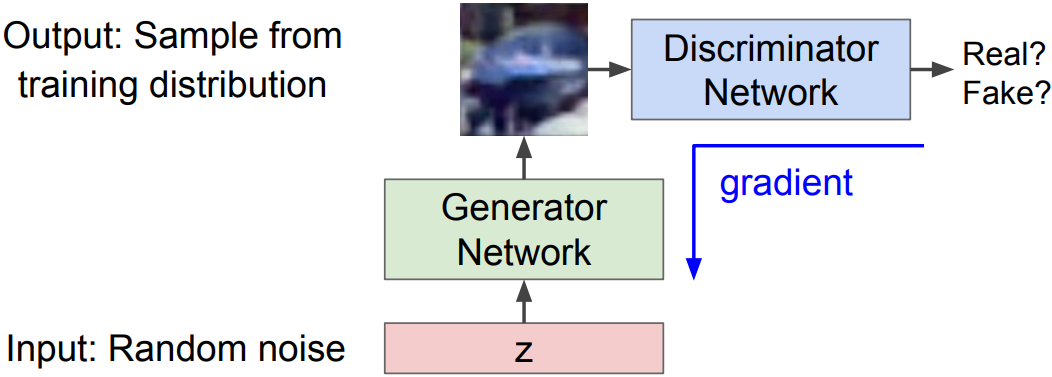
idea: Use a discriminator network to tell whether the generate image is within data distribution (“real”) or not

Training GANs: Two-player game

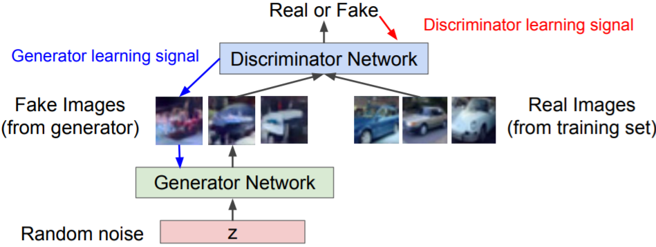
Discriminator network: try to distinguish between real and fake images
Generator network: try to fool discriminator by generating real-looking images

• Train jointly in minimax game;
  Minimax objective function:
  \(\mbox{min}_{\theta_g} \mbox{max}_{\theta_d}\left[\mathbb{E}_{x\sim {p_{data}}}\log D_{\theta_d}(x) + \mathbb{E}_{z\sim p(z)}\log(1-D_{\theta_d}(G_{\theta_g}(z))) \right]\)
  where $\theta_g$ is an objective for the generator objective and $\theta_d$ for the discriminator
  • $D_{\theta_d}(x)$: Discriminator outputs likelihood in (0,1) of real image
  • $D_{\theta_d}(G_{\theta_g}(z))$: Discriminator output for generated fake data G(z)
• Discriminator($\theta_d$) wants to maximize objective such that D(x) is close to 1(real) and D(G(z)) is close to 0(fake)
• Generator($\theta_g$) wants to minimize objective such that D(G(z)) is close to 1(to fool discriminator)

We alternate the minimax objection function with:

1. Gradient ascent on discriminator
   \(\mbox{max}_{\theta_d}\left[\mathbb{E}_{x\sim p_{data}}\log D_{\theta_d}(x) + \mathbb{E}_{z\sim p(z)}\log(1-D_{\theta_d}(G_{\theta_g}(z))) \right]\)
2. 1) Gradient descent on generator
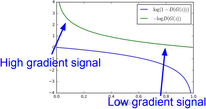
   \(\mbox{min}_{\theta_g}\mathbb{E}_{z\sim p(z)}\log(1-D_{\theta_d}(G_{\theta_g}(z)))\)
   • In practice, optimizing this generator objective does not work well;
     When sample is likely fake, want to learn from it to improve generator (move to the right on X axis), but gradient near 0 in X axis is relatively flat; Gradient signal is dominated by region where sample is already good(near 1).
     

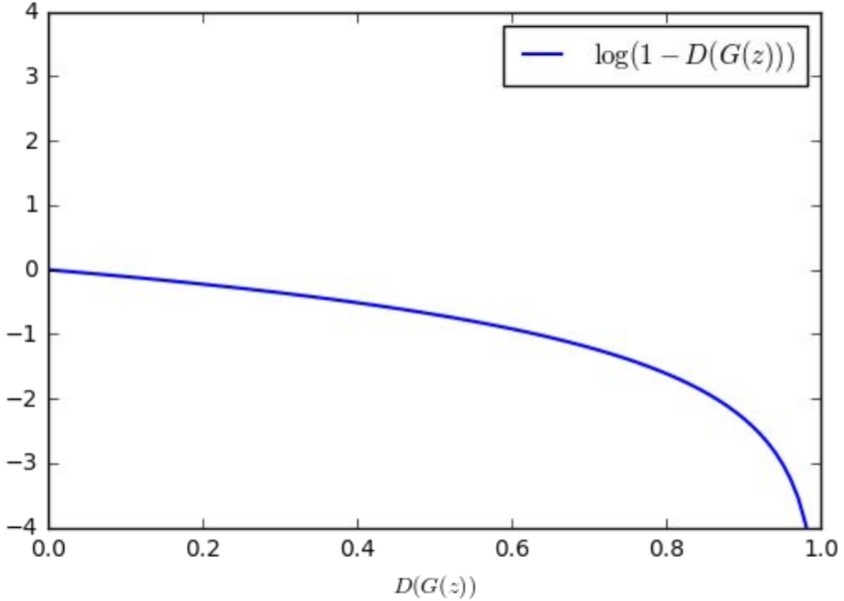
   2) Instead: Gradient ascent on generator, different objective
   \(\mbox{max}_{\theta_d}\mathbb{E}_{z\sim p(z)}\log(D_{\theta_d}(G_{\theta_g}(z)))\)

   • Rather than minimizing likelihood of discriminator being correct, maximize likelihood of discriminator being wrong. Same objective of fooling discriminator, but now higher gradient signal for bad samples.
     

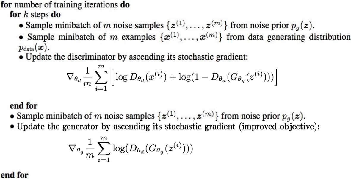
• GAN training Algorithm
  

• After training, use generator network to generate new images

GAN: Convolutional Architectures

• Generator is an upsampling network with fractionally-strided convolutions
  Discriminator is a convolutional network

• Architecture guidelines for stable Deep Conv GANs

  • Replace any pooling layers with strided convolutions(discriminator) and fractional-strided convolutions(generator).
  • Use batchnorm in both network.
  • Remove fully connected hidden layers for deeper architecture.
  • Use ReLU activation in generator for all layers except for the output, which uses Tanh.
  • Use LeakyReLU activation in the discriminator for all layers.

GAN: Interpretable Vector Math

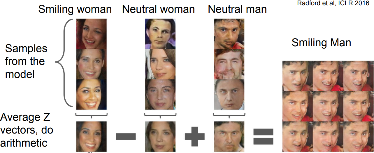
• works similar to a language model

2017: Explosion of GANs

• “The GAN Zoo”, https://github.com/hindupuravinash/the-gan-zoo
• check https://github.com/soumith/ganhacks for tips and tricks for training GANs

Scene graphs to GANs

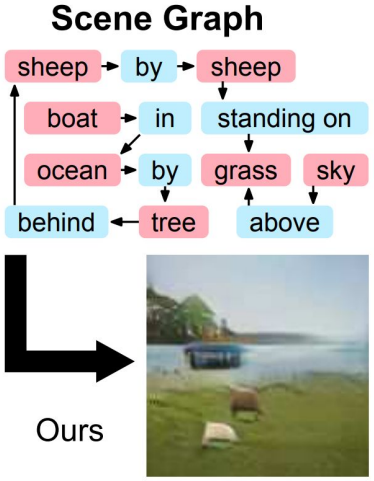
• Specifying exactly what kind of image you want to generate. The explicit structure in scene graphs provides better image generation for complex scenes.

Summary: GANs

• Don’t work with an explicit density function

• Take game-theoretic approach: learn to generate from training distribution through 2-player game

• Pros:
  • Beautiful, state-of-the-art samples
• Cons:
  • Trickier / more unstable to train
  • Can’t solve inference queries such as $p(x)$, $p(z\vert x)$
• Active areas of research:
  • Better loss functions, more stable training (Wasserstein GAN, LSGAN, many others)
  • Conditional GANs, GANs for all kinds of applications
• Useful Resources on Generative Models
  CS236: Deep Generative Models (Stanford)
  CS 294-158 Deep Unsupervised Learning (Berkeley)