Attention with RNNs

Image Captioning using spatial features

Input: Image I
Output: Sequence y $= y_1, y_2, \ldots, y_T$
Encoder: $h_0 = f_W(z)$, where z is spatial CNN features, $f_W(\cdot)$ is an MLP
Decoder: $y_t = g_v(y_{t-1}, h_{t-1}, c)$, where context vector c is often $c=h_0$

Problem: Input is “bottlenecked” through c; especially in a long descriptions. Model needs to encode everything it wants to say within c

Attention idea: New context vector c_t at every time step
Each context vector will attend to different image regions

• Alignment scores(scalars): $H \times W$ matrix e
  $e_{t,i,j} = f_{\mbox{att}}(h_{t-1}, z_{i,j})$
  where $f_{\mbox{att}}(\cdot)$ is an MLP
• Normalize to get attention weights:
  $a_{t,:,:} = \mbox{softmax}(e_{t,:,:})$,
  $0<a_{t,i,j}<1$, attention values sum to 1
• Compute context vector c: multiply CNN features and Attention weights
  $c_t = \sum_{i,j} a_{t,i,j} z_{t,i,j}$
• Decoder: $y_t = g_v(y_{t-1}, h_{t-1}, \color{red}{c_t})$

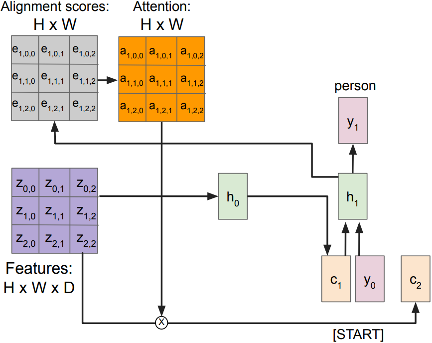
Each timestep of decode uses a different context vector that looks(attend) at different parts of the input image. This entire process is differentiable; model chooses its own attention weights. No attention supervision is required.

Similar tasks in NLP - Language translation example

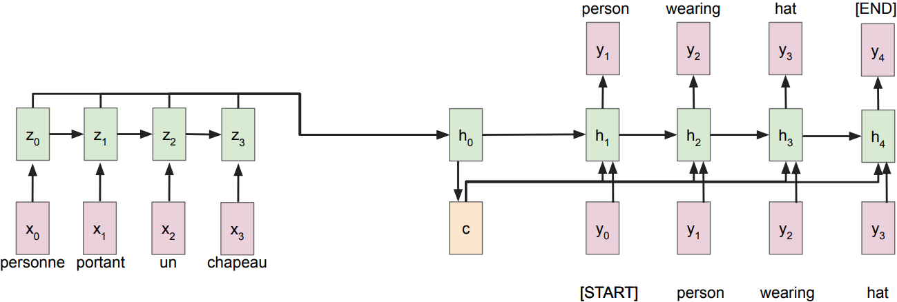
Vanilla Encoder-Decoder setting:

• Input: sequence x $= x_1, x_2, \ldots, x_T$
• Output: sequence y $= y_1, y_2, \ldots, y_T$
• Encoder: $h_0 = f_W(z)$, where $z_t = \mbox{RNN}(x_t, u_{t-1})$, $f_W(\cdot)$ is MLP, u is the hidden RNN state
• Decoder: $y_t = g_v(y_{t-1}, h_{t-1}, c)$, where context vector c is often $c=h_0$

Attention in NLP

• Alignment scores(scalars):
  $e_{t,i} = f_{\mbox{att}}(h_{t-1}, z_t)$, where $f_{\mbox{att}}(\cdot)$ is an MLP
• Normalize to get attention weights:
  $a_{t,:} = \mbox{softmax}(e_{t,:})$,
  $0<a_{t,i}<1$, attention values sum to 1
• Compute context vector c:
  $c_t = \sum_i a_{t,i} z_{t,i}$
• Decoder: $y_t = g_v(y_{t-1}, h_{t-1}, \color{red}c_t)$

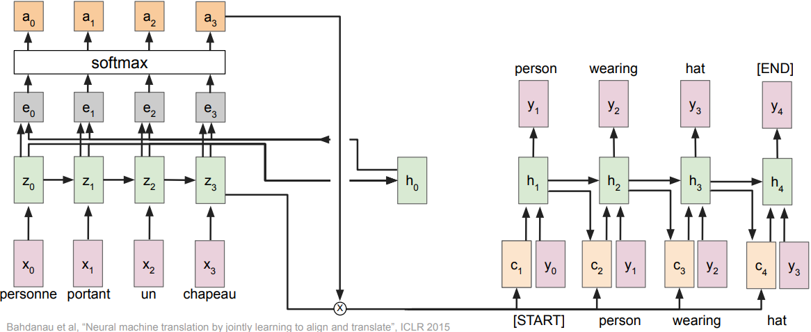
Heatmap: visualization of attention weights; without any attention supervision, model learns different word orderings for different languages

General Attention Layer

Attention in image captioning before

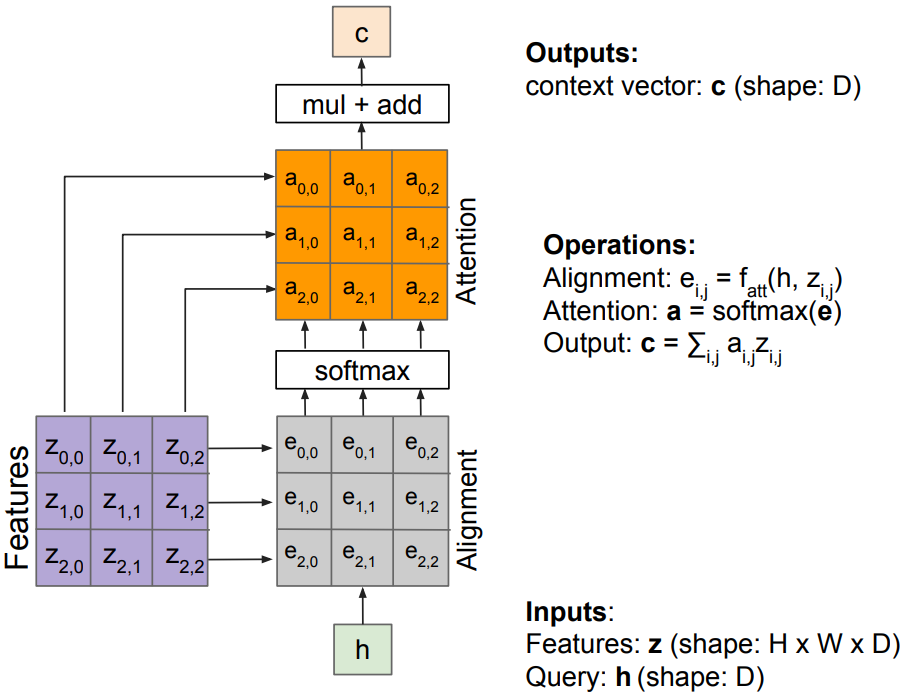
Single query setting

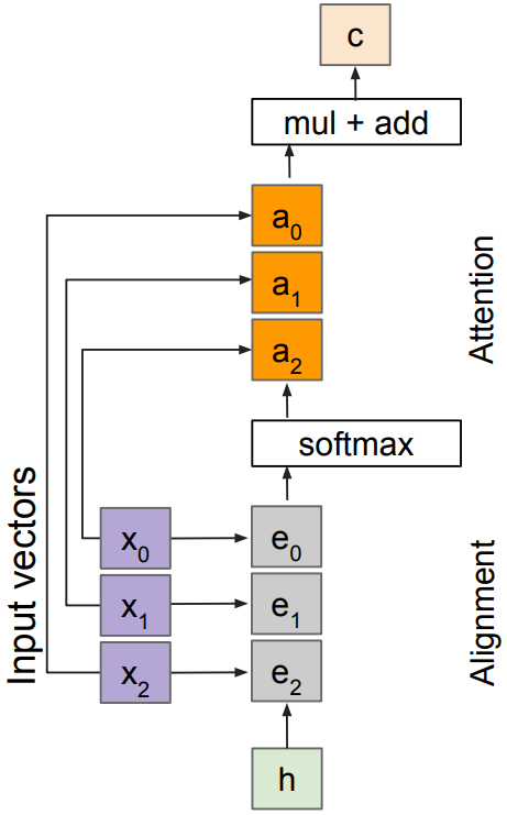
Inputs

• input vectors: x(shape: $N\times D$)
  Attention operation is permutation invariant; produces the same output regardless of the order of elements(features) in the input vector. Stretch $H\times W = N$ into N vectors, transform $H\times W\times D$ features into $N\times D$ input vectors x(similar to attention in NLP).
• Query: h(shape: D)

Operations

• Alignment
  • Change $f_{\mbox{att}}(\cdot)$ to a simple dot product:
    $e_i = h\cdot x_i$; only works well with key & value transformation trick
  • Change $f_{\mbox{att}}(\cdot)$ to a scaled dot product:
    $e_i = h\cdot x_i / \sqrt{D}$;
    Larger dimensions means more terms in the dot product sum. So, the variance of the logits is higher. Large magnitude(length) vectors will produce much higher logits. Then, the post-softmax distribution(e) has lower-entropy(high uncertainty) assuming logits are I.I.D. Ultimately, these large magnitude vectors will cause softmax to peak and assign very little weight to all others. To reduce this effect, divide by $sqrt{D}$.
• Attention: $\mathbf{a} = \mbox{softmax}(\mathbf{e})$
• Output: $\mathbf{c} = \sum_i a_i x_i$

Outputs
- context vector: c(shape: D)

Multiple query setting

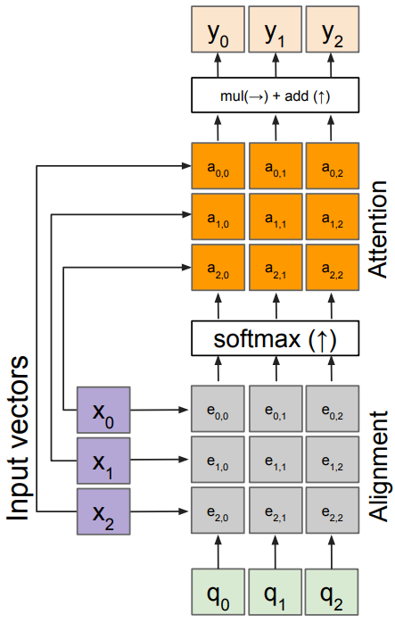
Inputs

• input vectors: x(shape: $N\times D$)
• Queries: q(shape: $M\times D$); multiple query vectors

Operations

• Alignment: $e_{i,j} = q_j\cdot x_i / \sqrt{D}$
• Attention: $\mathbf{a} = \mbox{softmax}(\mathbf{e})$
• Output: $y_j = \sum_i a_{i,j} x_i$

Outputs

• context vectors: y(shape: D);
  each query creates a new output context vector

Weight layers added

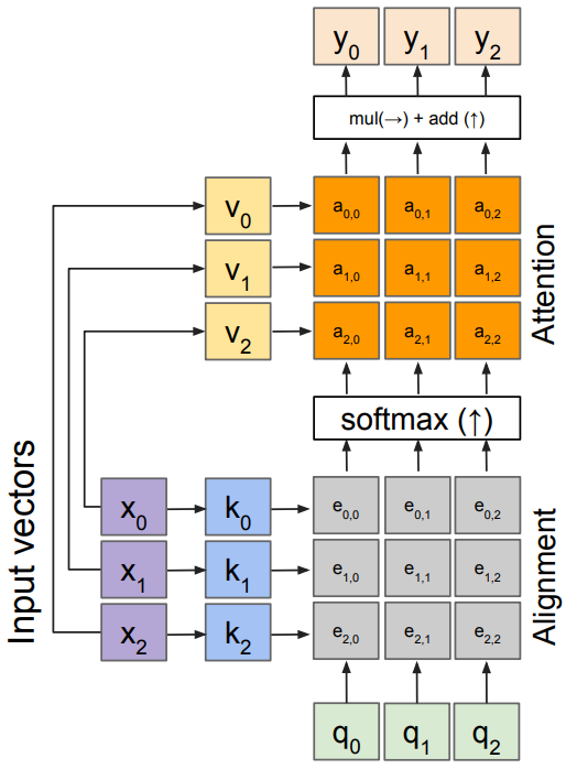
Notice that the input vectors x are used for both the alignment(e) and attention calculations(y); We can add more expressivity to the layer by adding a different FC layer before each of the two steps. The input and output dimensions can now change depending on the key and value FC layers.

Inputs

• input vectors: x(shape: $N\times D$)
• Queries: q(shape: $M\times D_k$)

Operations

• Key vectors: $\mathbf{k} = \mathbf{x}W_k$
• Value vectors: $\mathbf{v} = \mathbf{x}W_v$
• Alignment: $e_{i,j} = q_j\cdot k_i / \sqrt{D}$
• Attention: $\mathbf{a} = \mbox{softmax}(\mathbf{e})$
• Output: $y_j = \sum_i a_{i,j} v_i$

Outputs

• context vectors: y(shape: $D_v$);

Self attention layer

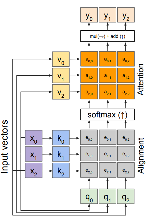
Recall that the query vector was a function of the input vectors; Encoder $h_0=f_W(z)$, where z is spatial CNN features, $f_W(\cdot)$ is an MLP. We can calculate the query vectors from the input vectors, defining a “self-attention” layer. No input query vectors anymore, instead query vectors are calculated using a FC layer.

Inputs

• input vectors: x(shape: $N\times D$)

Operations

• Key vectors: $\mathbf{k} = \mathbf{x}W_k$
• Value vectors: $\mathbf{v} = \mathbf{x}W_v$
• Query vectors: $\mathbf{q} = \mathbf{x}W_q$
• Alignment: $e_{i,j} = q_j\cdot k_i / \sqrt{D}$
• Attention: $\mathbf{a} = \mbox{softmax}(\mathbf{e})$
• Output: $y_j = \sum_i a_{i,j} v_i$

Outputs

• context vectors: y(shape: $D_v$)

Positional encoding

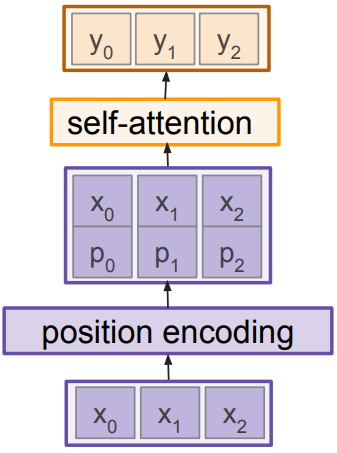
Self attention attends over sets of inputs; is permutation invariant. To encode the ordered sequences(e.g. language, image), concatenate special positional encoding $p_j$ to each input vector $x_j$.

$\mathit{pos}: N\rightarrow R^d$ to process the position j of the vector into a d-dimensional vector; $p_j = \mathit{pos}(j)$

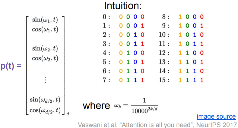
Desiderata of $\mathit{pos}(\cdot)$:

1. Should output a unique encoding for each time-step(word’s position in a sentence).
2. Distance between any two time-steps should be consistent across sentences with different lengths(variable inputs).
3. Model should generalize to longer sentences without any efforts. Its values should be bounded.
4. Must be deterministic.

Options for $\mathit{pos}(\cdot)$:

1. Learn a lookup table:
   • Learn parameters to use for $\mathit{pos}(t)$ for $t \in [0,T)$
   • Lookup table contains $T\times d$ parameters
2. Design a fixed function with the desiderata
   

Masked self-attention layer

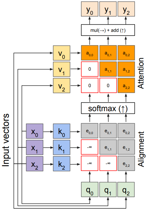
Manually set alignment scores to $-\infty$, prevent vectors from looking at future vectors.

Multi-head self attention layer

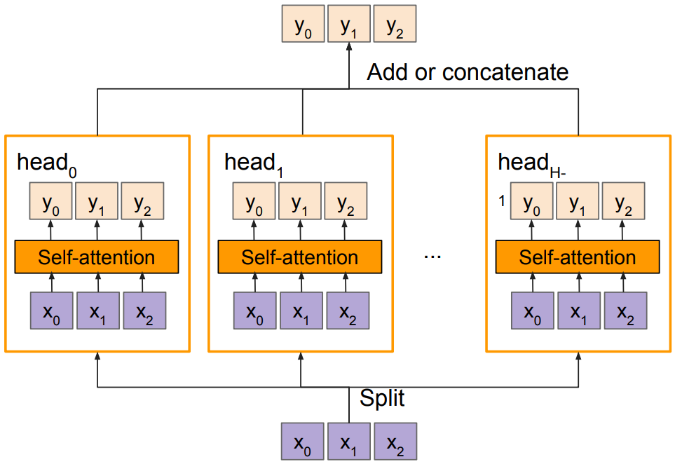
Multiple self-attention heads in parallel; similar to ensemble

Comparing RNNs to Transformers

RNNs
(+) LSTMs work reasonably well for long sequences.
(-) Expects an ordered sequences of inputs
(-) Sequential computation: subsequent hidden states can only be computed after the previous ones are done.

Transformers
(+) Good at long sequences. Each attention calculation looks at all inputs.
(+) Can operate over unordered sets or ordered sequences with positional encodings.
(+) Parallel computation: All alignment and attention scores for all inputs can be done in parallel.
(-) Requires a lot of memory: N x M alignment and attention scalers need to be calculated and stored for a single self-attention head.

Transformers

Image Captioning using transformers

• No recurrence at all

Input: Image I
Output: Sequence y $= y_1, y_2, \ldots, y_T$
Encoder: $c = T_W(z)$, where z is spatial CNN features, $T_W(\cdot)$ is the transformer encoder
Decoder: $y_t = T_D(y_{0:t-1}, c)$, where $T_D(\cdot)$ is the transformer decoder

The Transformer encoder block

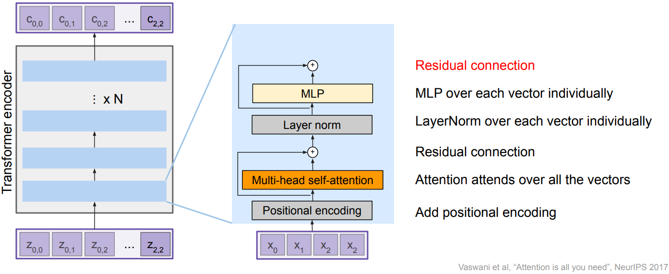
Inputs: Set of vectors x
Outputs: Set of vectors y

Self-attention is the only interaction between vectors; Layer norm and MLP operate independently per vector. Highly scalable, highly parallelizable, but high memory usage.

The Transformer Decoder block

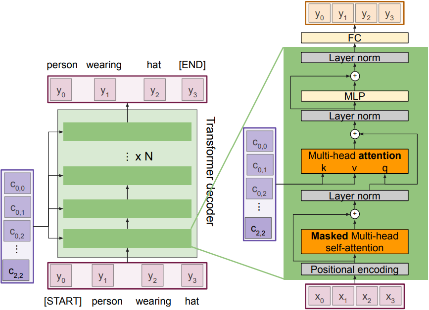
Inputs: Set of vectors x and Set of context vector c
Outputs: Set of vectors y

Masked Self-attention only interacts with past inputs(x, or previous output $y_{t-1}$). Multi-head attention block is NOT self-attention; it attends over the transformer encoder outputs. In this phase, we inject image features into the decoder. Highly scalable, highly parallelizable, but high memory usage.

Image Captioning using ONLY transformers

• Transformers from pixels to language
  Dosovitskiy et al, “An Image is Worth 16x16 Words: Transformers for Image Recognition at Scale”, ArXiv 2020 colab notebook link

• Note: in Google Colab - TPU runtime setting

import tensorflow as tf
import os

# TPU initialization
resolver = tf.distribute.cluster_resolver.TPUClusterResolver(tpu='grpc://' + os.environ['COLAB_TPU_ADDR'])

tf.config.experimental_connect_to_cluster(resolver)
tf.tpu.experimental.initialize_tpu_system(resolver)

strategy = tf.distribute.TPUStrategy(resolver)

# compile in strategy.scope
def create_model():
  return tf.keras.Sequential(
      [tf.keras.layers.Conv2D(256, 3, activation='relu', input_shape=(28, 28, 1)),
       tf.keras.layers.Conv2D(256, 3, activation='relu'),
       tf.keras.layers.Flatten(),
       tf.keras.layers.Dense(256, activation='relu'),
       tf.keras.layers.Dense(128, activation='relu'),
       tf.keras.layers.Dense(10)])

with strategy.scope():
  model = create_model()
  model.compile(optimizer='adam',
                loss=tf.keras.losses.SparseCategoricalCrossentropy(from_logits=True),
                metrics=['sparse_categorical_accuracy'])

Summary

• Adding attention to RNNs allows them to “attend” to different parts of the input at every time step
• The general attention layer is a new type of layer that can be used to design new neural network architectures
• Transformers are a type of layer that uses self-attention and layer norm.
  • It is highly scalable and highly parallelizable
  • Faster training, larger models, better performance across vision and language tasks
  • They are quickly replacing RNNs, LSTMs, and may even replace convolutions.