Linear Classifier (cont.)

• Todo:
  1. Define a loss function: how good the classifier is
  2. Optimization: efficient way of finding the parameters that minimize the loss function

• Loss function
  given a dataset of examples \(\left\{ (x_i,y_i) \right\}_{n=1}^N\)
  where $x_i$ is image and $y_i$ is (integer) label
  Average of loss over examples: \(L=\frac{1}{N}\sum_i L_i(f(x_i,W),y_i)\)

• Multiclass SVM loss:
  using the shorthand for the scores vector: $s = f(x_i,W)$
  \(L_i=\sum_{j\ne y_i}\mbox{max}(0,s_j-s_{y_i}+1)\)
  where +1 is a safety margin

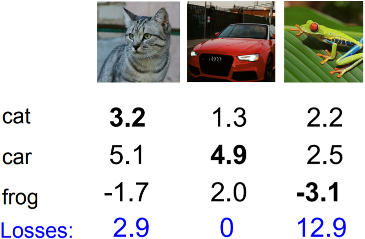
Q1: What happens to loss if car scores decrease by 0.5 for this training example?
L = max(0,0.8-4.4+1) + max(0,1.5-4.4+1) = 0
Result will not be changed; SVM hinge loss is robust to small change of scores.

Q2: what is the min/max possible SVM loss $L_i$?
The possible minimum value of SVM loss is 0 and maximum value is $\infty$.

Q3: At initialization W is small so all s ≈ 0. What is the loss $L_i$, assuming N examples and C classes?
C-1 the number of classes minus 1.
(Sanity check for weight initialization)

Q4: What if the sum was over all classes? (including $j = y_i$)
All losses increased by 1, so as the average loss over full dataset. In this case, the minimum value of loss will be 1. What we want is to minimize the loss function and that’s why we remove the class $s_j=s_{y_i}$ to set it 0.

Q5: What if we used mean instead of sum?
Because a loss function is to find optimizing parameters, rescaling loss has no effect to the result.

Q6: What if we used squared function of \(L_i=\sum_{j\ne y_i}\mbox{max}(0,s_j-s_{y_i}+1)^2\)
A squared hinge loss can be better at finding optimizing parameters W. If the observation is close to the answer, it will reflect the loss much smaller than original hinge loss.

def L_i_vectorized(x,y,W):  
	scores = W.dot(x)  
	margins = np.maximum(0, scores -scores[y] +1)
	margins[y]=0
	loss_i = np.sum(margins)
	return loss_i

$f(x,W) = Wx$
\(L=\frac{1}{N}\sum_{i=1}^N \mbox{max}(0,f(x_i;W)_j -f(x_i;W)y_i +1)\)

Q7: Suppose that we found a W such that $L = 0$. Is this W unique?
No. 2W is also has $L=0$. W not a unique solution.
$\rightarrow$ How do we choose between W and 2W?

• Regularization: introduce penalty term $\lambda R(W)$ on L(W)
  L2 regularization: $R(W)=\sum_k\sum_l W_{k,l}^2$; likes to spread out the weights
  L1 regularization: $R(W)=\sum_k\sum_l |W_{k,l}|$
  Elastic net (L1 + L2): $R(W) = \sum_k\sum_l\beta W_{k,l}^2 + |W_{k,l}|$
  Dropout, Batch normalization, Stochastic depth, fractional pooling, etc.

• Why regularize?
  Express preferences over weights
  Make the model simple so it works on test data
  Improve optimization by adding curvature

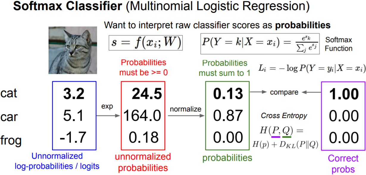
Softmax classifier(Multinomial Logistic Regression)

The information content(also called the surprisal or self-information) is described as $h(E) = -\log P(E)$. For a discrete random variable X, its entropy(or expected; mean information) $H(X) = -\sum_{i=1}^N p_i \log p_i$. Cross-entropy is an approximaton of q to p is to minimizing KL(p|q), while the Kullback–Leibler divergence as $D_{KL}(P||Q)=\sum_y P(y)\log\frac{P(y)}{Q(y)} = \sum_y P(y)\log P(y) - \sum_y P(y)\log Q(y)$. Thus, cross entropy loss $L = -\sum_y P(y)\log Q(y)$.

Q1: What is the min/max possible softmax loss $L_i$?
min 0 to max $\infty$

Q2: At initialization all $s_j$ will be approximately equal; what is the softmax loss $L_i$, assuming C classes?
$-\log(1/C)=\log C$

Recap

For some dataset of $(x,y)$, a score function $s = f(x;W)$, a loss function $L_i$,
Full loss \(L=\frac{1}{N}\sum_{i=1}^N L_i + R(W)\)

Optimization

• Strategy: Follow the slope
  In 1-dimension, the derivative of a function:
  \(\frac{df(x)}{dx}=\lim_{n\to 0}\frac{f(x+h)-f(x)}{h}\)
  In multiple dimensions, the gradient is the vector of (partial derivatives) along each dimension.
  The slope in any direction is the dot product of the direction with the gradient. The direction of steepest descent is the negative gradient.
  The loss is just a function of W, what we want is $\nabla_w L$
  In practice: Always use analytic gradient, but check implementation with numerical gradient. This is called a gradient check.

• Stochastic Gradient Descent(SGD)
  Full sum expensive when N is large. Approximate su using a minibatch of examples (32 / 64 / 128 common)

# Vanilla Minibatch Gradient Descent
while True:
	data_batch = sample_training_data(data,256)  
	weights_grad = evaluate_gradient(loss_fun, data_batch, weights)
	weights += - step_size * weights_grad