cs231n - Lecture 4. Neural Networks and Backpropagation
Image Features
- Problem: Linear Classifiers are not very powerful
- Visual Viewpoint: Linear classifiers learn one template per class
- Geometric Viewpoint: Linear classifiers can only draw linear decision boundaries
-
Image Features: Motivation
After applying feature transform, points can be separated by linear classifier
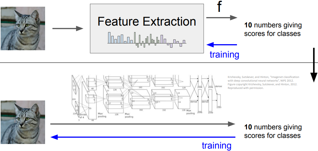
$f(x,y) = (r(x,y), \theta(x,y))$ - Image Features vs. ConvNets

Neural Networks
-
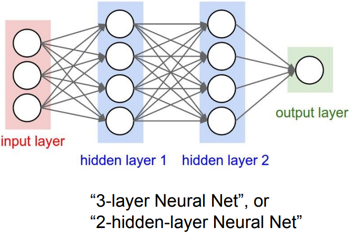
Neural networks, also called Fully connected networks(FCN) or sometimes multi-layer perceptrons(MLP)
(Before) Linear score function:
\(\begin{align*}& f=Wx \\ & x\in\mathbb{R}^D, W\in\mathbb{R}^{C\times D} \end{align*}\)
$\rightarrow$ 2-layer Neural Network:
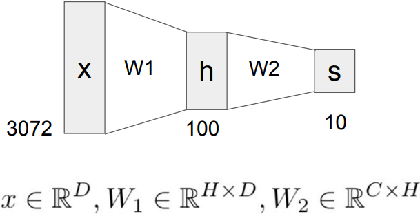
\(\begin{align*}& f=W_2 \mbox{max}(0,W_1 x) \\ & x\in\mathbb{R}^D, W_1\in\mathbb{R}^{H\times D}, W_2\in\mathbb{R}^{C\times H} \end{align*}\)
$\rightarrow$ or 3-layer Neural Network:
\(f=W_3\mbox{max}(0,W_2 \mbox{max}(0,W_1 x)) \\ \vdots\)
(In practice we will usually add a learnable bias at each layer as well) -
Neural networks: hierarchical computation

Learning 100s of templates instead of 10 and share templates between classes -
Why is max operator important?
The function $\mbox{max}(0,z)$ is called the activation function.
Q: What if we try to build a neural network without one?
A: We end up with a linear classifier again!
$f=W_2 W_1 x, W_3=W_1 W_2, f = W_3 x$ -
Activation functions
ReLU($\mbox{max}(0,z)$) is a good default choice for most problems
Others: Sigmoid, tanh, Leaky ReLU, Maxout, ELU, etc. -
Neural networks: Architectures
Example feed-forward computation of a neural network

# forward-pass of a 3-layer neural network:
f = lambda x: 1.0/(1.0 + np.exp(-x)) # activation function (use sigmoid)
x = np.random.randn(3,1) # random input vector of three numbers (3x1)
h1 = f(np.dot(W1, x) + b1) # calculate first hidden layer activations (4x1)
h2 = f(np.dot(W2, h1) + b2) #calculate second hidden layer activations (4x1)
out = np.dot(W3, h2) + b3 #output neuron (1x1)
Full implementation of training a 2-layer Neural Network:
import numpy as np
from numpy.random import randn

N, D_in, H, D_out = 64, 1000, 100, 10	# Define the network
x, y = randn(N, D_in), randn(N, D_out)
w1, w2 = randn(D_in, H), randn(H, D_out)

for t in range(2000):					# Forward pass
	h = 1 / (1 + np.exp(-x.dot(w1)))
	y_pred = h.dot(w2)
	loss = np.square(y_pred - y).sum()
	print(t, loss)

	grad_y_pred = 2.0 * (y_pred - y)	# Calculate the analytical gradients
	grad_w2 = h.T.dot(grad_y_pred)
	grad_h = grad_y_pred.dot(w2.T)
	grad_w1 = x.T.dot(grad_h * h * (1-h))

	w1 -= 1e-4 * grad_w1				# Gradient descent
	w2 -= 1e-4 * grad_w2
-
Plugging in neural networks with loss functions
$s = f(x;W_1,W_2) = W_2\mbox{max}(0,W_1 x)$ Nonlinear score function
$L_i = \sum_{j\ne y_i}\mbox{max}(0,s_j-s_{y_i}+1)$ SVM Loss on predictions
$R(W)=\sum_k W_k^2$ Regularization
$L=\frac{1}{N}\sum_{i=1}^N L_i + \lambda R(W_1) + \lambda R(W_2)$ Total loss: data loss + regularization -
Problem: How to compute gradients?
If we can compute partial derivaties, then we can learn $W_1$ and $W_2$.
Backpropagation
-
Chain rule:
\(\begin{align*} \frac{\partial f}{\partial y}=\frac{\partial f}{\partial q} \frac{\partial q}{\partial y} \mbox{Upstream gradient} \times \mbox{Local gradient} \end{align*}\) -
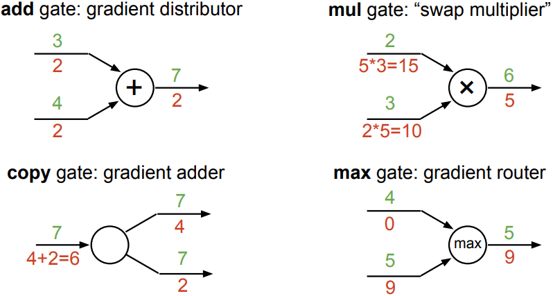
Patterns in gradient flow
