Review: Main idea of word2vec

• Start with random word vectors
• Iterate through each word in the whole corpus
• Try to predict surrounding words using word vectors: $P(o\mid c) = \frac{\exp(u_o^T v_c)}{\sum_{w \in V}\exp(u_w^T v_c)}$
• Learning: Update vectors so they can predict actual surrounding words better
• Doing no more than this, this algorithm learns word vectors that capture well word similarity and meaningful directions in a wordspace.
  
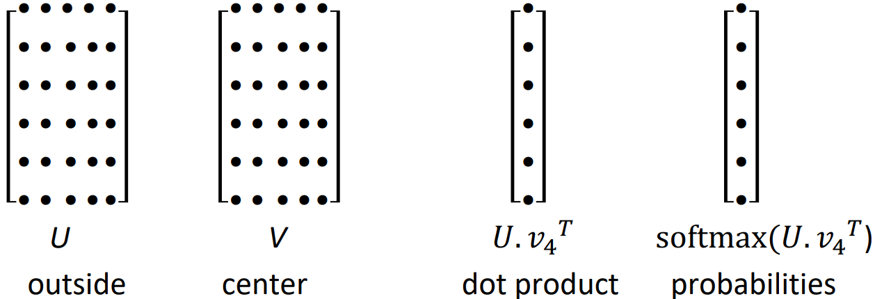
• A “bag of words” model; doesn’t actually pay any attention to word order or position. The model makes the same predictions at each position; the probability estimate would be the same if it is next to the center word or a bit further away.

• We want a model that gives a reasonably high probability estimate to all words that occur in the context(at all often)

• Word2vec maximizes objective function by putting similar words nearby in high dimensional vector space

Optimization: Gradient Descent

• To learn good word vectors: minimize a cost function $J(\theta)$
• Gradient Descent is an algorithm to minimize $J(\theta)$ by changing $\theta$
• idea: from current value of $\theta$, calculate gradient of $J(\theta)$, then take small step in the direction of negative gradient. Repreat.
  
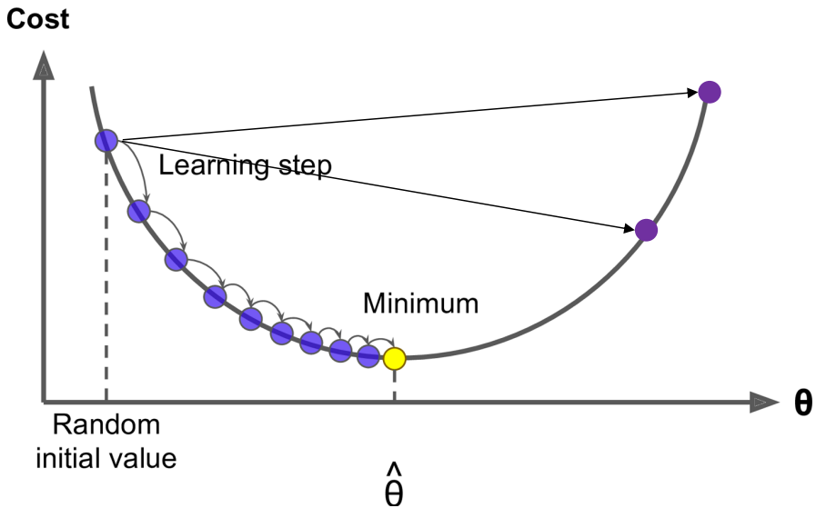
• Algorithm:

  while True:
    theta_grad = evaluate_gradient(J, corpus, theta)
    theta = theta - alpha * theta_grad
  

Stochastic Gradient Descent

• Problem: $J(\theta)$ is a function of all windows in the corpus (often, billions!); so $\nabla_\theta J(\theta)$ is very expensive to compute
• Solution: Stochastic gradient descent(SGD)
  • Repeatedly sample windows, and update after each one, or each small batch
• Algorithm:

  while True:
    window = sample_window(corpus)
    theta_grad = evaluate_gradient(J, window, theta)
    theta = theta - alpha * theta_grad
  

• Stochastic gradients with word vectors (Aside)
  • iteratively take gradients at each such window for SGD
  • But in each window, we only have at most 2m + 1 words,
    so $\nabla_\theta J(\theta)$ is very sparse:
    \(\nabla_\theta J_t(\theta) = \begin{bmatrix} 0 \\ \vdots \\ \nabla_{v_{\text{like}}} \\ \vdots 0 \\ \nabla_{u_I} \\ \vdots \\ \nabla_{u_{\text{learning}}} \\ \vdots \end{bmatrix} \in \mathbb{R}^{2dV}\)
  • We might only update the word vectors that actually appear.
  • Solution: either you need sparse matrix update operations to only update certain rows(in most DL packages) of full embedding matrices U and V, or you need to keep around a hash for word vectors.
    
  • If you have millions of word vectors and do distributed computing, it is important to not have to send gigantic updates around.

2b. Word2vec algorithm family: More details

• Why two vectors? $\rightarrow$ Easier optimization. Average both at the end
  • But can implement the algorithm with just one vector per word, and it works slightly better, but it makes the algorithm much more complicated.
• Two model variants:
  1. Skip-grams(SG)
     Predict context(“outside”) words (position independent) given center word
  2. Continuous Bag of Words(CBOW)
     Predict center word from (bag of) context words
     We presented: Skip-gram model
• Additional efficiency in training:
  • Negative sampling
    So far: Focus on naive softmax(simpler, but expensive training method)

The skip-gram model with negative sampling(SGNS)

• The normalization term is computationally expensive, especially on the denominator of $P(o\mid c)$.
• Main idea: train binary logistic regressions for a true pair (center word and a word in its context window) versus several noise pairs (the center word paired with a random word)
• From paper: “Distributed Representations of Words and Phrases and their Compositionality” (Mikolov et al. 2013)
• Overall objective function(to maximize):
  \(J(\theta) = \frac{1}{T}\sum_{t=1}^T J_t(\theta)\)
  \(J_t(\theta) = \log\sigma(u_o^T u_c) + \sum_{i=1}^k \mathbb{E}_{j~P(w)}\left[ \log\sigma(-u_j^T v_c) \right]\)
  where the logistic/sigmoid function: $\sigma(x) = \frac{1}{1+ e^{-x}}$
• We maximize the probability of two words co-occuring in first log and minimize probability of noise words:
  $J_{\text{neg-sample}}(u_o, v_c, U) = -\log \sigma(u_o^T v_c) - \sum_{k\in { \text{K sampled indicies} }} \log \sigma(-u_k^T v_c)$
• We take k negative samples (using word probabilities)
• Maximize probability that real outside word appears, minimize probability that random words appear around center word
• Another trick: sample with $P(w) = U(w)^{3/4} / Z$, the unigram distribution $U(w)$ raised to the $3/4$ power (We provide this function in the starter code)
• The power makes less frequent words be sampled more often

Why not capture co-occurrence counts directly?

• Building a co-occurrence matrix X
  • 2 options: windows vs. full document
  • Window: Similar to word2vec, use window around each word and captures some syntactic and semantic information
    
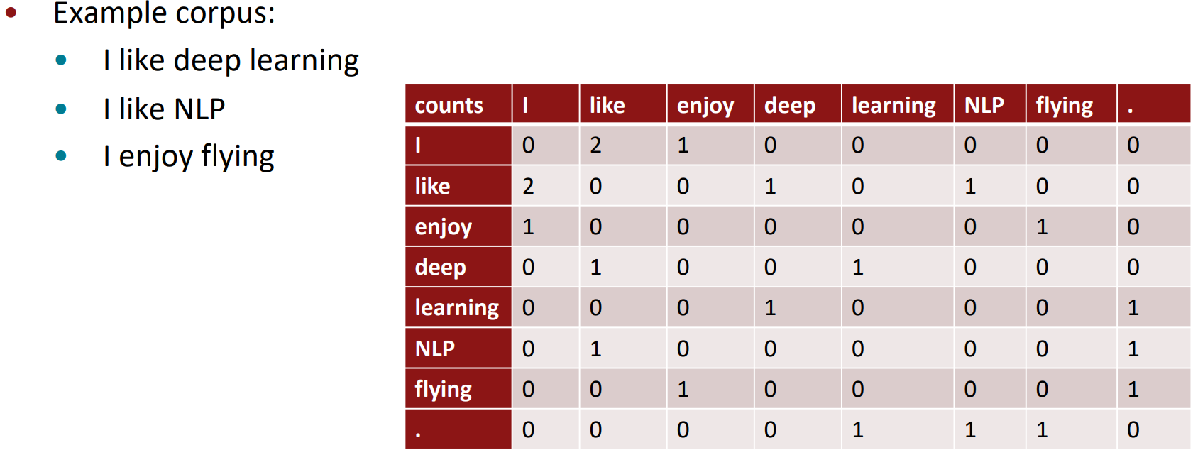
  • Word-document co-occurrence matrix will give general topics (all sports terms will have similar entries) learning to “Latent Semantic Analysis”; in tasks like information retrieval

Co-occurrence vectors

• Simple count co-occurrence vectors
  • Vectors increase in size with vocabulary
  • Very high dimensional: require a lot of storage (though sparse)
  • Subsequent classification models have sparsity issues $\rightarrow$ Models are less robust
• Low-dimensional vectors
  • idea: store “most” of the important information in a fixed, small number of directions: a dense vector
  • Usually 25-1000 directions, similar to word2vec
  • How to reduce the dimensionality?

Classic Method: Dimensionality Reduction on X

• Singular Value Decomposition of co-occurrence matrix X
  Factorizes X into $U\Sigma V^T$, where U and V are orthonormal
  
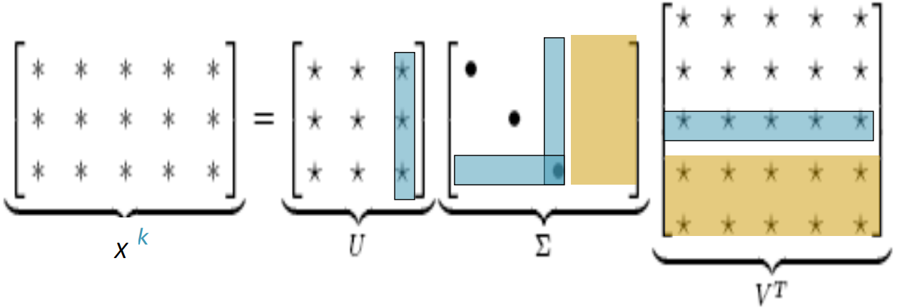
  Corresponding to the columns without singular values in $\Sigma$, bottom rows in $V^T$ are ignored. The singular values inside the diagonal matrix $\Sigma$ are ordered from largest down to smallest. Retaining only k singular values, in order to generalize, the lower dimensional representation $\hat{X}$ is the best rank k approximation to X, in terms of least squares.

Hacks to X (several used in Rohde et al. 2005 in COALS)

• Running an SVD on a raw count co-occurrence matrix works poorly; In the mathematical assumptions of SVD, we are expecting to have normally distributed errors. But there are exceedingly common words like “a”, “the”, and “and”, and there is a very large number of rare words.

• Scaling the counts in the cells can help a lot
  • Problem: function words(the, he, has) are too frequent $\rightarrow$ syntax has too much impact. Some fixes:
    • log the frequencies
    • $min(X,t)$, with $t\approx 100$
    • ignore the function words
• Ramped windows that count closer words more than further away words
• Use Pearson correlations instead of counts, then set negative values to 0
• Etc.
• Result:
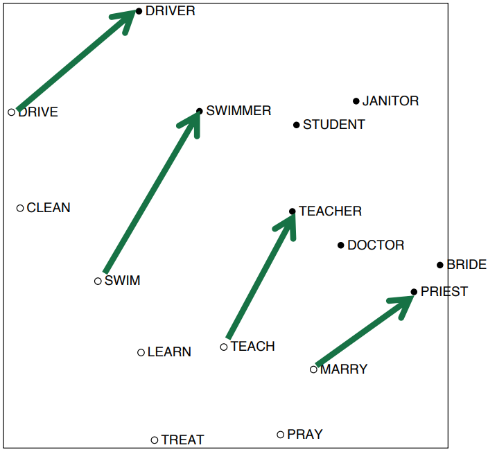
  Interesting semantic patterns emerge in the scaled vectors; something like a word vector analogies.
  

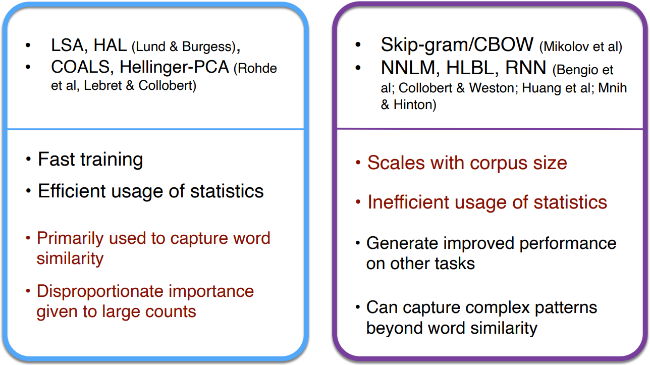
Towards GloVe: Count based vs. direct prediction

Encoding meaning components in vector differences

• Pennington, Socher, and Manning, EMNLP 2014
• What properties needed to make vector analogies work?

• Crucial insight: Ratios of co-occurrence probabilities can encode meaning components
  
  

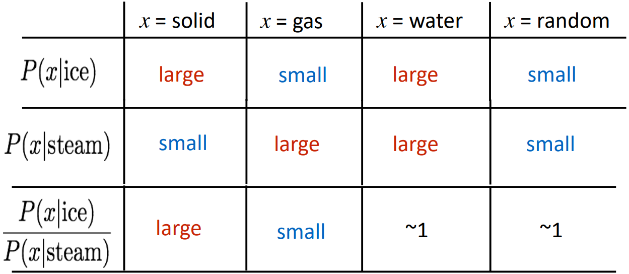
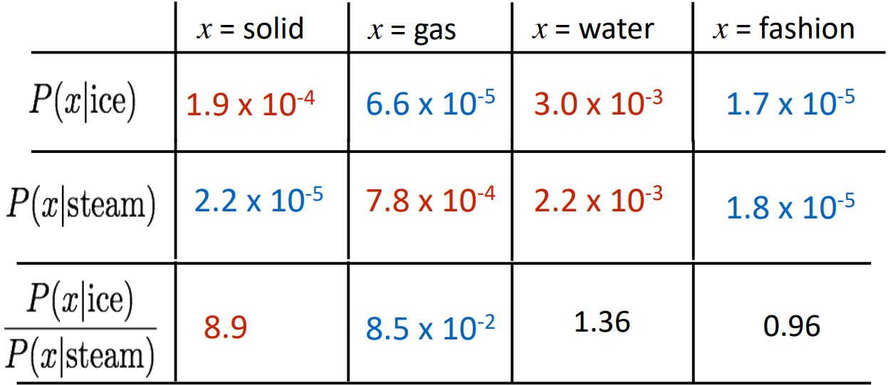
• Q: How can we capture ratios of co-occurrence probabilities as linear meaning components in a word vector space?
• A: Log-bilinear model: the dot product between two word vectors attempts to approximate the log of the probability of co-occurrence; \(w_i \cdot w_j = \log P(i|j)\)
  $\rightarrow$ with vector differences \(w_x \cdot (w_a - w_b) = \log \frac{P(x\mid a)}{P(x \mid b)}\)

Combining the best of both worlds: GloVe

• Pennington, Socher, and Manning, EMNLP 2014
• With \(w_i \cdot w_j = \log P(i|j)\),
  explicit loss function \(J = \sum_{i,j=1}^V f(X_{ij})(w_i^T \tilde{w}_j + b_i + \tilde{b}_j - \log X_{ij})^2\)
  to make the dot product to be similar to the log of the co-occurrence. To not have very common words dominate, capped the effect of high word counts using $f$ function. Optimize J directly on the co-occurrence count matrix.
  • Fast training
  • Scalable to hugh corpora
  • Good performance even with small corpus and small vectors

How to evaluate word vectors?

• Related to general evaluation in NLP: intrinsic vs. extrinsic
• Intrinsic:
  • Evaluation on a specific/intermediate subtask
  • Fast to compute
  • Helps to understand that system
  • Not clear if really helpful unless correlation to real task is established
• Extrinsic:
  • Evaluation on a real task
  • Can take a long time to compute accuracy
  • Unclear if the subsystem is the problem or its interaction or other subsystems
  • If replacing exactly one subsystem with another improves accuracy $\rightarrow$ Winning!

Intrinsic word vector evaluation

• Word Vector Analogies
  |a:b :: c:?| $\rightarrow$ $d = \text{argmax}_i \frac{(x_b -x_a +x_c)^T x_i}{\lVert x_b -x_a +x_c\rVert}$
  (e.g. man:woman :: king:?)
• Evalute word vectors by how well their cosine distance after addition captures intuitive semantic and syntactic analogy questions
• Discarding the input words from the search!
• Problem: What if the information is there but not linear?

GloVe Visualizations

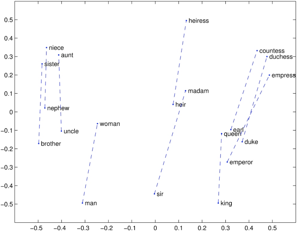
Analogy evaluation and hyperparameters

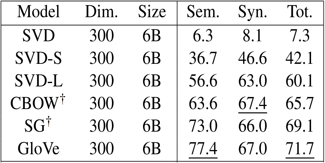
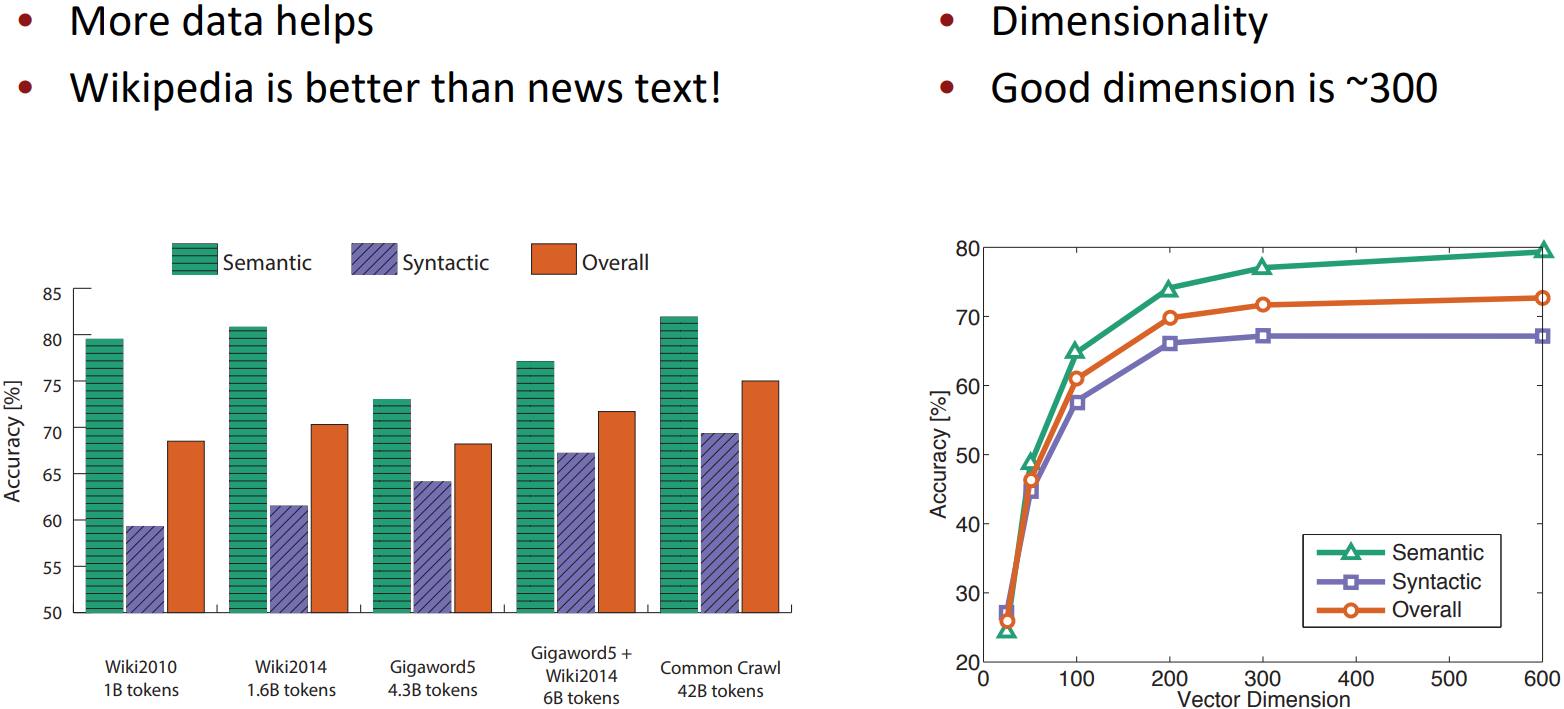
Another intrinsic word vector evaluation

• Word vector distances and their correlation with human judgements
• Example dataset: WordSim353 http://www.cs.technion.ac.il/~gabr/resources/data/wordsim353/

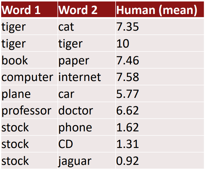
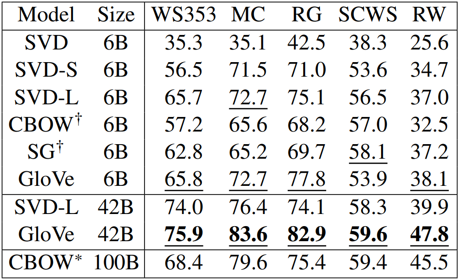
• Some ideas from Glove paper have been shown to improve skip-gram(SG) model also (e.g., average both vectors)

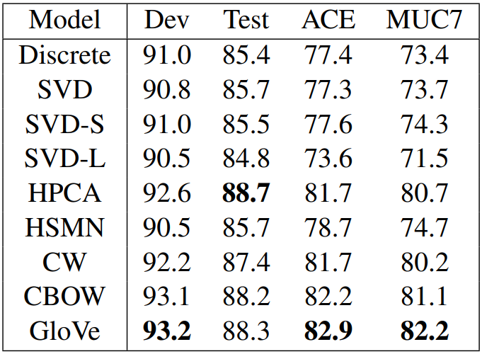
Extrinsic word vector evaluation

• All subsequent NLP tasks
• One example where good word vectors should help directly: named entity recognition: identifying references to a person, organization or location

Word senses

• Most words have lots of meanings
  • Especially common words
  • Especially words that have existed for a long time
• Does one vector caputre all these meanings or do we have a mess?

“Linear Algebric Structure of Word Senses, with Applications to Polysemy”, Arora, …, Ma, …, TACL 2018

• Different senses of a word reside in a linear superposition(weighted sum) in standard word embeddings like word2vec
• \(v_{\text{pike}} = \alpha_1 v_{\text{pike}_2} + \alpha_2 v_{\text{pike}_2} + \alpha_3 v_{\text{pike}_3}\)
  where $\alpha_1 = \frac{f_1}{f_1+f_2+f_3}$, etc., for frequency f
• Surprising result:
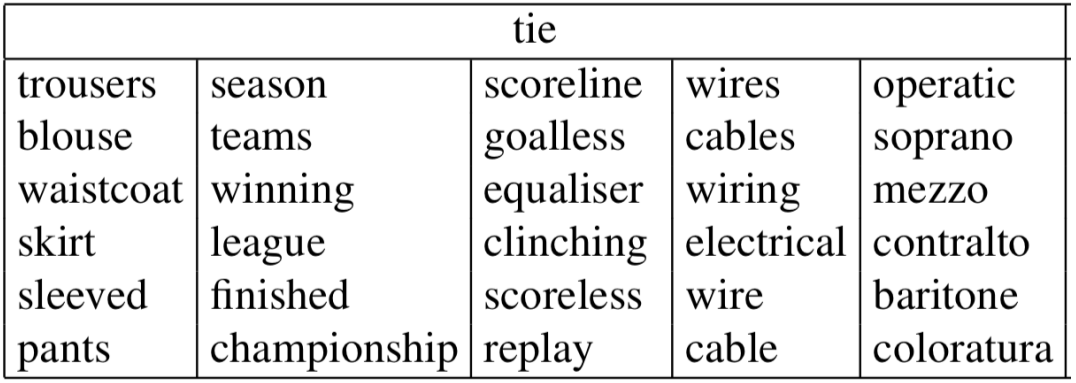
  Commonly, it is impossible to reconstruct the original components from their sum, but, because of ideas from sparse coding you can actually separate out the senses(providing they are relatively common)!