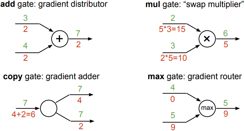
cs224n - Lecture 3. Backprop and Neural Networks
Named Entity Recognition(NER)
- Task: find and classify names in text
- Possible uses:
- Tracking mentions of particular entities in documents
- For question answering, answers are usually named entities
- Often followed by Named Entity Linking/Canonicalization into Knowledge Base
Simple NER: Window classification using binary logistic classifier
-
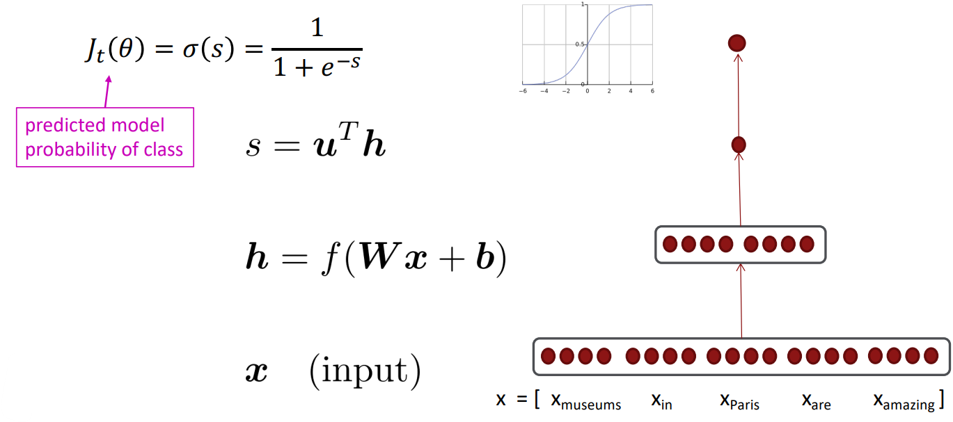
Using word vectors, build a context window of word vectors, then pass through a neural network and feed it to logistic classifier.
- idea: classify each word in its context window of neighboring words
- Train logistic classifier on hand-labeled data to classify center word {yes/no} for each class based on a concatenation of word vectors in a window
- In practice, we usually use multi-class softmax
- Example: Classify “Paris” as +/- location(binary for is_location) in context of sentence with window length 2:
sentence $=$ “$\mbox{ the museums in Paris are amazing to see . }$” $x_{\text{window}} = [x_{\text{museums}}\quad x_{\text{in}}\quad x_{\text{Paris}}\quad x_{\text{are}}\quad x_{\text{amazing}}]^T$ - Resulting vector $x_{\text{window}} = x\in \mathbb{R}^{5d}$, a column vector.
- To classify all words: run classifier for each class on the vector centered on each word in the sentence
Computing Gradients by Hand
- Matrix calculus: Fully vectorized gradients
- “Multivariable calculus is just like single-variable calculus if you use matrices”
- Much faster and more usful than non-vectorized gradients
- But doing a non-vectorized gradient can be good for intuition; partial derivative for one parameter
- Vector gradient
Given a function with 1 output and n inputs
$f(x) = f(x_1, x_2, \ldots, x_n)$
Its gradient is a vector of partial derivatives w.r.t each input
\(\frac{\partial f}{\partial x} = \left[\frac{\partial f}{\partial x_1}, \frac{\partial f}{\partial x_2}, \cdots, \frac{\partial f}{\partial x_n} \right]\) -
Jacobian Matrix: Generalization of the Gradient
Given a function with m outputs and n inputs
$f(x) = [f_1(x_1, x_2, \ldots, x_n), \ldots, f_m(x_1, x_2, \ldots, x_n)]$
It’s Jacobian is an $m \times n$ matrix of partial derivatives
\(\begin{align*} \frac{\partial f}{\partial x} = \begin{bmatrix} \frac{\partial f_1}{\partial x_1} & \cdots & \frac{\partial f_1}{\partial x_n} \\ \vdots & \ddots & \vdots \\ \frac{\partial f_m}{\partial x_1} & \cdots & \frac{\partial f_m}{\partial x_n} \end{bmatrix} \end{align*}\) $\quad\quad$ \(\begin{align*}\left( \frac{\partial f}{\partial x} \right)_{ij} = \frac{\partial f_i}{\partial x_j}\end{align*}\) - Chain Rule
- For composition of one-variable functions: multiply derivatives
$z = g(y)$, $y = f(x)$
\(\begin{align*}\frac{dz}{dx} = \frac{dz}{dy}\frac{dy}{dx}\end{align*}\) - For multiple variables at once: multiply Jacobians
$h = f(z)$
$z = Wx + b$
\(\begin{align*}\frac{\partial h}{\partial x} = \frac{\partial h}{\partial z}\frac{\partial z}{\partial x} = \cdots\end{align*}\)
- For composition of one-variable functions: multiply derivatives
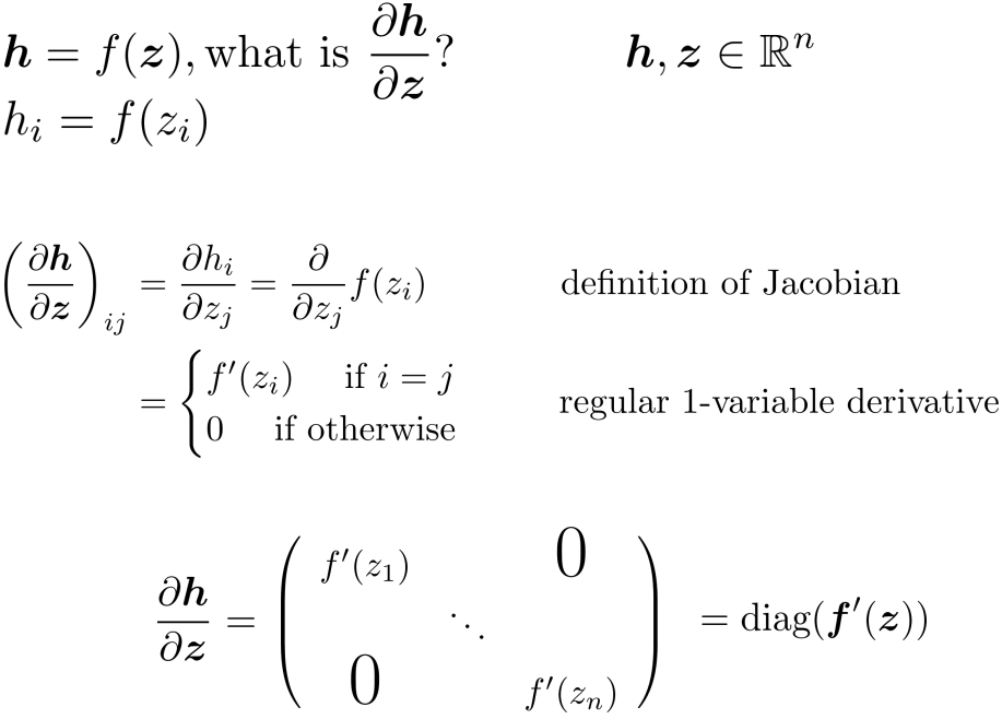
- Example Jacobian: Elementwise activation function
- Other Jacobians
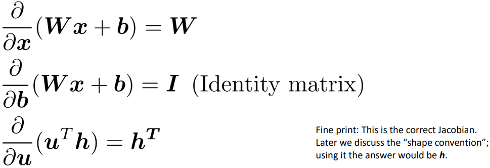
- Write out the Jacobians
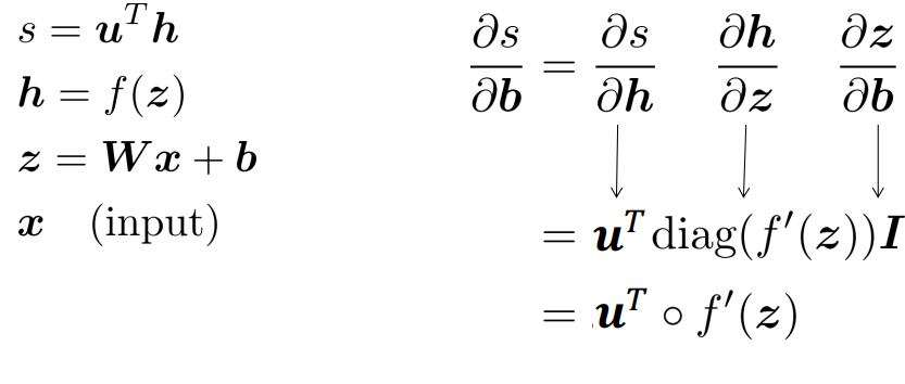
- Derivative with respect to Matrix: Output shape
for $\frac{\partial s}{\partial W}$, output $s$ is a scalar and input $W \in \mathbb{R}^{n\times m}$: 1 by nm Jacobian?
$\rightarrow$ is inconvenient to do \(\theta^{\text{new}} = \theta^{\text{old}} - \alpha\nabla_\theta J(\theta)\) gradient descent.- Instead, use the shape convention: the shape of the gradient is the shape of the parameters
n by m matrix \(\begin{align*}\frac{\partial s}{\partial W} = \begin{bmatrix} \frac{\partial s}{\partial W_{11}} & \cdots & \frac{\partial s}{\partial W_{1m}} \\ \vdots & \ddots & \vdots \\ \frac{\partial s}{\partial W_{n1}} & \cdots & \frac{\partial s}{\partial W_{nm}} \end{bmatrix}\end{align*}\) - $\frac{\partial s}{\partial W} = \delta\frac{\partial z}{\partial W}$
$z = Wx + b$
\(\begin{align*} \frac{\partial s}{\partial W} &= \delta^T x^T \\ & = \begin{bmatrix} \delta_1 \\ \vdots \\ \delta_n \end{bmatrix} [x_1, \ldots, x_m] = \begin{bmatrix} \delta_1 x_1 & \cdots & \delta_1 x_m \\ \vdots & \ddots & \vdots \\ \delta_n x_1 & \cdots & \delta_n x_m \end{bmatrix} \end{align*}\)
denote that $\delta$ is local error signal at z and x is local input signal.
- Instead, use the shape convention: the shape of the gradient is the shape of the parameters
What shape should derivatives be?
- Two options:
- Use Jacobian form as much as possible, reshape to follow the shape convention at the end:
- at the end transpose $\frac{\partial s}{\partial b}$ to make the derivative a column vector, resulting in $\delta^T$
- Always follow the shape convention
- Look at dimensions to figure out when to transpose and/or reorder terms
- The error message $\delta$ that arrives at a hidden layer has the same dimensionality as that hidden layer
- Use Jacobian form as much as possible, reshape to follow the shape convention at the end:
Backpropagation: Chain Rule
- Other trick:
re-use derivatives computed for higher layers in computing derivatives for lower layers to minimize computation
