cs224n - Lecture 5. Language Models and RNNs
How do we gain from a neural dependency parser?
- So far…
Transition based dependency parsers were an efficient linear time method for giving the syntactic structure of natural language text.
Worked pretty well before neural nets came along.
$\color{red}{(-)}$ They worked with indicator features, specifying some condition and then checking whether it was true of a configuration. Problems of those features are:- Problem #1: sparse
- Problem #2: incomplete
- Problem #3: expensive computation
More than 95% of parsing time is consumed by feature computation
- Neural Approach:
Start with the same configuration of a stack and a buffer, run exactly the same transition sequence but with a dense vector.
A neural dependency parser(Chen and Manning, 2014)
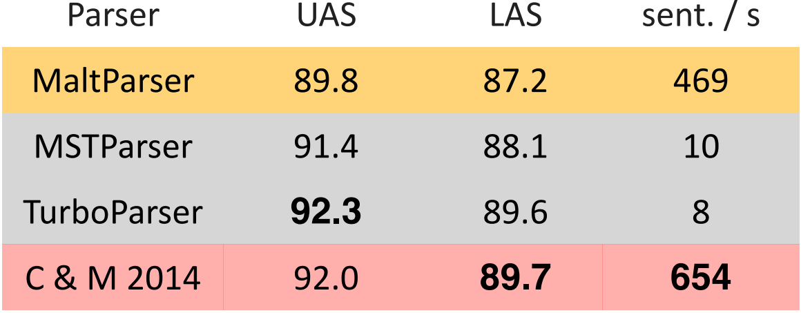
- Results on English parsing to Stanford Dependencies:
- Unlabeled attachment score (UAS) = head
- Labeled attachment score (LAS) = head and label
- 2% more accurate than the symbolic dependency parser
- noticeably faster
First win: Distributed Representations
- Represent each word as a d-dimensional dense vector (i.e., word embedding)
- Similar words are expected to have close vectors.
- Meanwhile, part-of-speech tags(POS) and dependency labels are also represented as d-dimensional vectors.
- The smaller discrete sets also exhibit many semantical similarities.
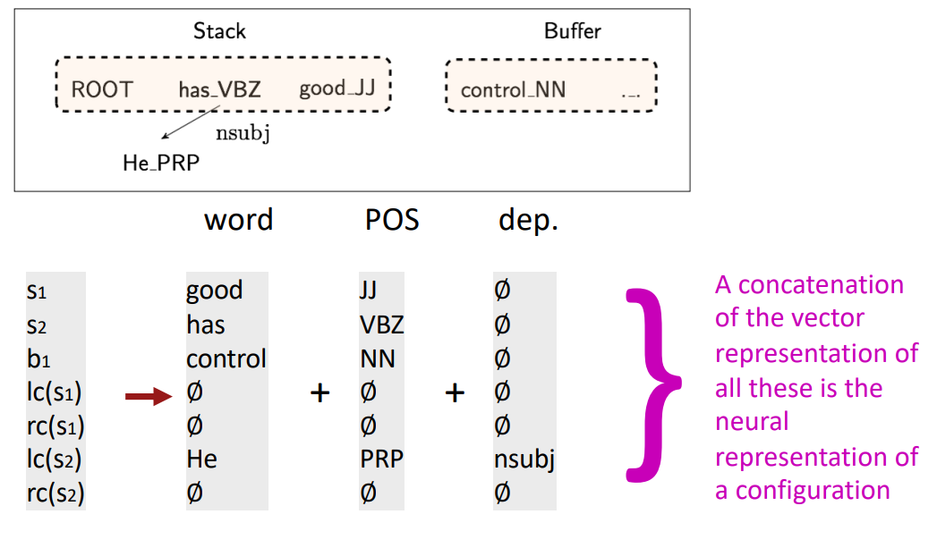
- Extracting Tokens & vector representations from configuration
- Extract a set of tokens based on the stack / buffer positions:
Second win: Deep Learning classifiers are non-linear classifiers
-
A softmax classifier assigns classes $y\in C$ based on inputs $x \in \mathbb{R}^d$ via the probability:
\(\begin{align*} p(y\mid x) = \frac{\exp(W_y . x)}{\sum_{c=1}^C \exp(W_c . x)} \end{align*}\) - We train the weight matrix $W \in \mathbb{R}^{C\times d}$ to minimize the neg. log loss: $\sum_i - \log p(y_i\mid x_i)$ (a.k.a. “cross entropy loss”)
-
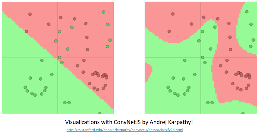
Traditional ML classifiers (including Naive Bayes, SVMs, logistic regression and softmax classifier) are not very powerful classifiers: they only give linear decision boundaries; limiting, unhelpful when a problem is complex.
- Neural networks can learn much more complex functions with nonlinear decision boundaries.
- Non-linear in the original space, linear for the softmax at the top of the neural network
Simple feed-forward neural network multi-class classifier
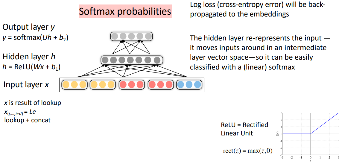
Neural Dependency Parser Model Architecture
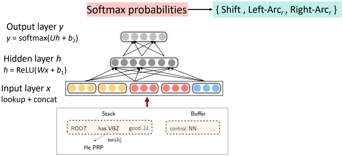
Dependency parsing for sentence structure
- C & M 2014 showed that neural networks can accurately determine the structure of sentences, supporting meaning interpretation

- It was the first simple, successful neural dependency parser
- The dense representations (and non-linear classifier) let it outperform other greedy parsers in both accuracy and speed
Further developments in transition-based neural dependency parsing
-
Improvements Bigger, deeper networks with better tuned hyperparameters
Beam search
Global, conditional random field (CRF)-style inference over the decision sequence -
Leading to SyntaxNet and the Parsey McParseFace model(2016):
“The World’s Most Accurate Parser”
https://ai.googleblog.com/2016/05/announcing-syntaxnet-worlds-most.html
Graph-based dependency parsers
- Compute a score for every possible pair; dependency (choice of head) for each word
- Doing this well requires more than just knowing the two words
- We need good “contextual” representations of each word token, which we will develop in the coming lectures
- Repeat the same process for each other word; find the best parse (MST algorithm)
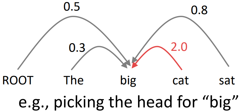
A Neural graph-based dependency parser
-
Dozat and Manning 2017; Dozat, Qi, and Manning 2017
- This paper revived interest in graph-based dependency parsing in a neural world
- Designed a biaffine scoring model for neural dependency parsing
- Also crucially uses a neural sequence model
- Great results, but slower than the simple neural transition-based parsers
- There are $n^2$ possible dependencies in a sentence of length $n$

A bit more about neural networks
Regularization
-
A full loss function includes regularization over all parameters $\theta$, e.g., L2 regularization:
\(\begin{align*} J(\theta) = \frac{1}{N}\sum_{i=1}^N -\log \left( \frac{e^{f_{y_i}}}{\sum_{c=1}^C e^{f_c}} \right) + \lambda\sum_k \theta_k^2 \end{align*}\) -
Classic view: Regularization works to prevent overfitting when we have a lot of features (or later a very powerful/deep model, etc.)
-
Now: Regularization produces models that generalize well when we have a “big” model
- We do not care that our models overfit on the training data, even though they are hugely overfit
Dropout
-
[Srivastava, Hinton, Krizhevsky, Sutskever, & Salakhutdinov 2012/JMLR 2014]
-
Preventing Feature Co-adaptation = Good Regularization Method
- Training time: at each instance(or batch) of evaluation (in online SGD-training), randomly set 50% of the inputs to each neuron to 0
- Test time: halve the model weights (because we now keep twice as many active neurons)
(Except usually only drop first layer inputs a little (~15%) or not at all) - Prevents feature co-adaptation: A feature cannot only be useful in the presence of particular other features
- In a single layer: A kind of middle-ground between Naive Bayes (where all feature weights are set independently) and logistic regression models (where weights are set in the context of all others)
- Can be thought of as a form of model bagging (i.e., like an ensemble model)
- Nowadays usually thought of as strong, feature-dependent regularizer
[Wager, Wang, & Liang 2013]
“Vectorization”
- E.g., looping over word vectors versus concatenating them all into one large matrix and then multiplying the softmax weights with that matrix:
from numpy import random
N = 500 # number of windows to classify
d = 300 # dimensionality of each window
C = 5 # number of classes
W = random.rand(C, d)
wordvectors_list = [random.rand(d, 1) for i in range(N)]
wordvectors_one_matrix = random.rand(d, N)

%timeit [W.dot(wordvectors_list[i]) for i in range(N)]
%timeit W.dot(wordvectors_one_matrix)
- Always try to use vectors and matrices rather than for loops; the speed gain goes from 1 to 2 orders of magnitude with GPUs.
Non-linearities, old and new
- logistic(“sigmoid”)
\(\begin{align*} f(z) = \frac{1}{1+\exp(-z)}\end{align*}\) - tanh
\(\begin{align*} f(z) = \tanh(z) = \frac{e^z - e^{-z}}{e^z + e^{-z}}\end{align*}\)
tanh is just a rescaled and shifted sigmoid(2x as steep, [-1, 1]):
$tanh(z) = 2 \text{logistic}(2z) - 1$ - hard tanh
\(\begin{align*} \text{PHardTanh}(x) = \begin{cases} -1 & \mbox{ if } x < -1 \\ x & \mbox{ if } -1 \le x \le 1 \\ 1 & \mbox{ if } x > 1 \end{cases}\end{align*}\) -
ReLU(Rectrified Linear Unit)
$\text{rect}(z) = \text{max}(z, 0)$ -
Others
Leaky ReLU / Parametric ReLU, Swish(Ramachandran, Zoph & Le 2017) - Both logistic and tanh are still used in various places(e.g., to get a probability), but are no longer the defaults for making deep networks
For building a deep network, first try ReLU - it trains quickly and performs well due to good gradient backflow
Parameter Initialization
- Initialize weights to small random values (i.e., not zero matrices)
To avoid symmetries that prevent learning/specialization - Initialize hidden layer biases to 0 and output (or reconstruction) biases to optimal value if weights were 0 (e.g., mean target or inverse sigmoid of mean target)
- Initialize all other weights $~ \text{Uniform}(–r, r)$, with $r$ chosen so numbers get neither too big or too small (later the need for this is removed with use of layer normalization)
- Xavier initialization has variance inversely proportional to fan-in $n_{in}$ (previous layer size) and fan-out $n_{out}$ (next layer size):
\(\begin{align*} Var(W_i) = \frac{2}{n_{in} + n_{out}} \end{align*}\)
Optimizers
- SGD will work just fine, but getting good results will often require hand-tuning the learning rate
- Sophisticated “adaptive” optimizers that scale the parameter adjustment by an accumulated gradient; Adam is fairly good, safe place to start in many cases
Learning Rates
- A constant learning rate. Start around $lr = 0.001$?
- It must be order of magnitude right – try powers of 10
Too big: model may diverge or not converge
Too small: model may not have trained by the assignment deadline
- It must be order of magnitude right – try powers of 10
- Better try learning rate decay
- By hand: : halve the learning rate every k epochs
- By a formula: $lr = lr_0 e^{-kt}$, for epoch $t$
- There are fancier methods like cyclic learning rates (q.v.)
- Fancier optimizers still use a learning rate but it may be an initial rate that the optimizer shrinks – so you may want to start with a higher learning rate
Language Modeling
- Language Modeling is the task of predicting what word comes next
-
More formally: given a sequence of words $x^{(1)}, x^{(2)}, \ldots, x^{(t)}$, compute the probability distribution of the next words $x^{(t+1)}$:
$P(x^{(t+1)} \mid x^{(t)}, \ldots, x^{(1)})$
where $x^{(t+1)}$ can be any word in the vocabulary \(V = \left\{ w_1, \ldots, w_{\lvert V \rvert} \right\}\) -
You can also think of a Language Model as a system that assigns probability to a piece of text
- For example, if we have some text $x^{(1)}, x^{(2)}, \ldots, x^{(T)}$, then the probability of this text (according to the Language Model) is:
\(\begin{align*} P(x^{(1)}, \ldots, x^{(T)}) &= P(x^{(1)}) \times P(x^{(2)}\mid x^{(1)}) \times \cdots \times P(x^{(T)}\mid x^{(T-1)}, \ldots, x^{(1)}) \\ &= \prod_{t=1}^T \underbrace{P(x^{(t)}\mid x^{(t-1)}, \ldots, x^{(1)})}_{\text{This is what our LM provides}} \end{align*}\)
n-gram Language Models
- Question: How to learn a Language Model?
- Answer(traditional, pre- Deep Learning): learn an n-gram Language Model
- Definition: A _n-gram__ is a chunk of n consecutive words.
- Idea: Collect statistics about how frequent different n-grams are and use these to predict next word.
- First we make a Markov assumption: $x^{(t+1)}$ depends only on the preceding n-1 words;
- Question: How do we get these n-gram and (n-1)-gram probabilities?
- Answer: By counting them in some large corpus of text
n-gram Language Models: Example
Suppose we are learning a 4-gram Language Model.
as the proctor started the clock, the students opened their w(target)
\(\begin{align*} P(\mathbf{w}|\text{students opened their}) = \frac{\text{count}(\text{students opened their } \mathbf{w})}{\text{students opened their}} \end{align*}\)
- For example, suppose that in the corpus:
- “students opened their” occurred 1000 times
- “students opened their books” occurred 400 times
$\rightarrow P(\text{books}|\text{students opened their}) = 0.4$ - “students opened their exams” occurred 100 times
$\rightarrow P(\text{exams}|\text{students opened their}) = 0.1$
Then, Should we have discarded the “proctor” context?
- Naive Bayes: a class specific unigram language model, counting individual words
Problems with n-gram Language Models
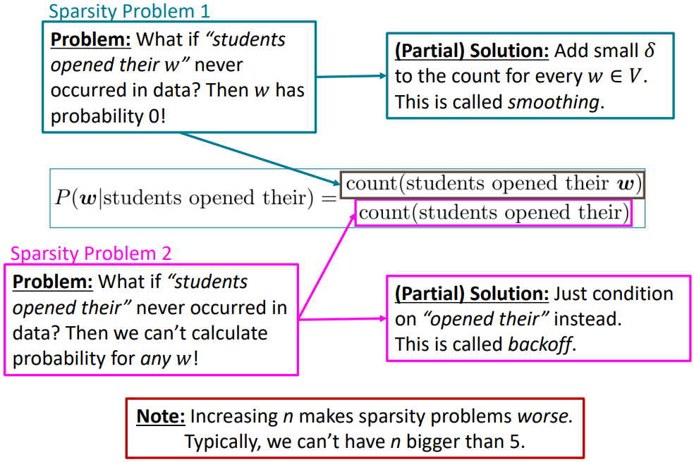
- Sparsity:
- Storage: Need to store count for all n-grams you saw in the corpus
Increasing n or increasing corpus increases model size
n-gram Language Models in practice
- You can build a simple trigram Language Model over a 1.7 million word corpus (Reuters) in a few seconds on your laptop
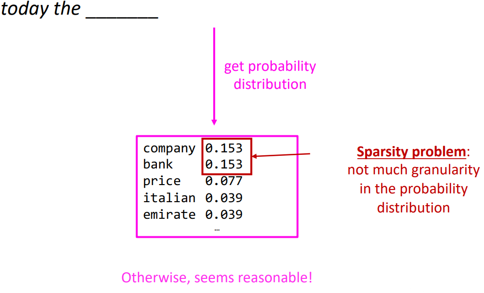
- You can also use a Language Model to generate text
- Get probability distribution, sample one. move forward and iterate.
- Results are incoherent. Need to consider more n words but increasing n worsens sparsity problem, and increases model size
How to build a neural Language Model?
- Recall the Language Modeling task:
- Input: sequence of words $x^{(1)}, x^{(2)}, \ldots, x^{(t)}$
- Output: prob dist of the next word $P(x^{(t+1)} \mid x^{(t)}, \ldots, x^{(1)})$
- Window-based neural model
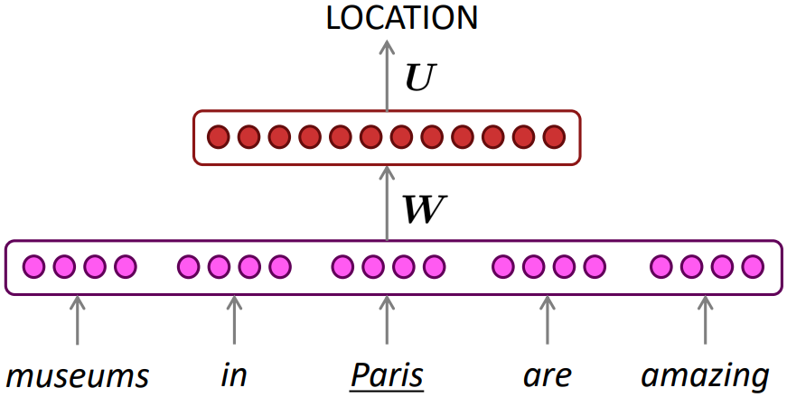
A fixed-window neural Language Model
Approximately: Y. Bengio, et al. (2000/2003): A Neural Probabilistic Language Model
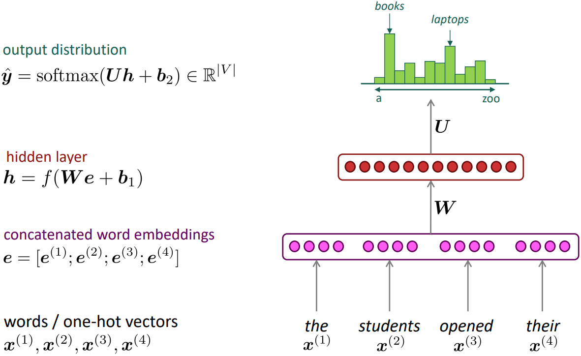
- Improvements over n-gram LM:
- No sparsity problem
- Don’t need to store all observed n-grams
- Remaining problems:
- Fixed window is too small
- Enlarging window enlarges $W$
- Window can never be large enough
- $x^{(1)}$ and $x^{(2)}$ are multiplied by completely different weights in $W$. No symmetry in how the inputs are processed.
$\rightarrow$ We need a neural architecture that can process any length input
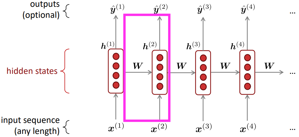
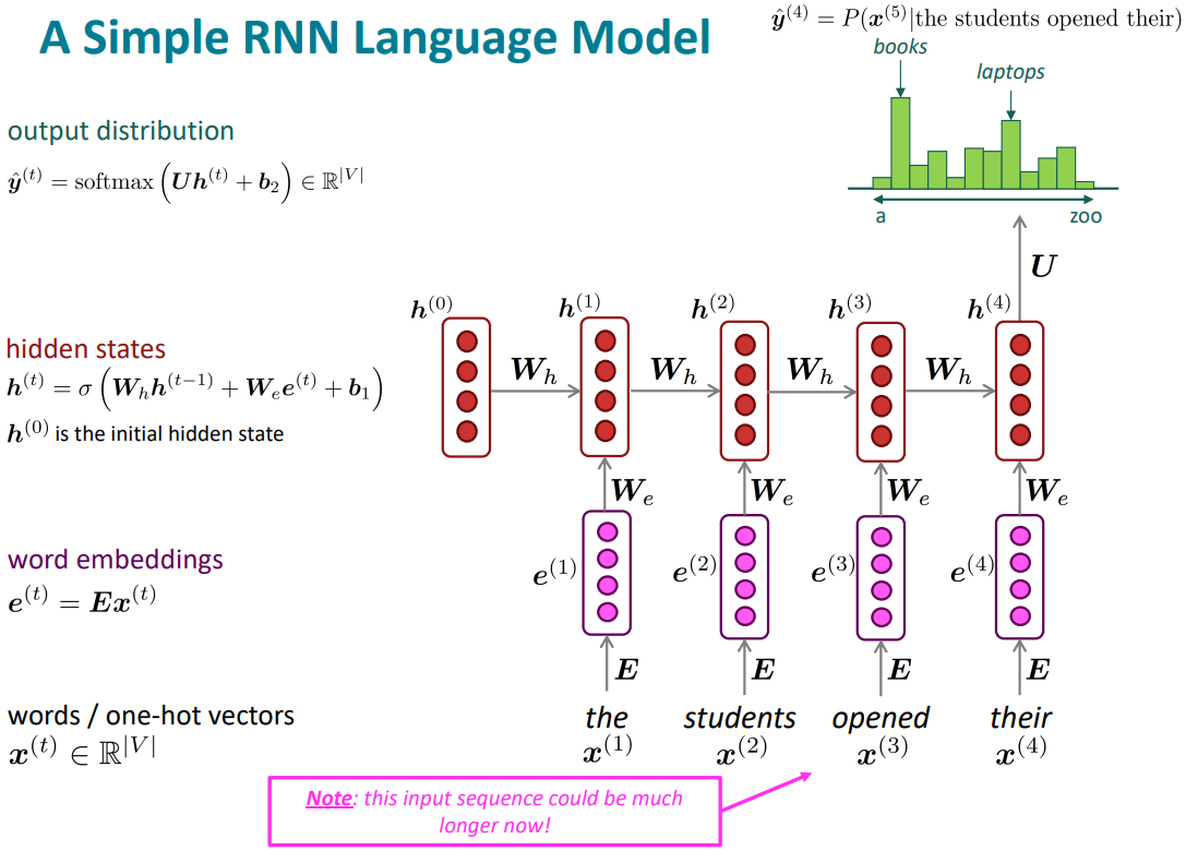
Recurrent Neural Networks (RNN)
- Core idea: Apply the same weights $W$ repeatedly
- RNN Advantages:
- Can process any length input
- Computation for step t can (in theory) use information from many steps back
- Model size doesn’t increase for longer input context
- Symmetry input process; same weights applied on every timestep
- RNN Disadvantages:
- Recurrent computation is slow
- In practice, difficult to access information from many steps back